This page was generated from docs/examples/2_mergingstats.ipynb. Interactive online version: .

HEWL S-SAD Merging Statistics

Merging statistics are a useful means to assess data quality in crystallography. However, each statistic has inherent shortcomings. For example, R-merge will appear inflated if the multiplicity is high, and the Pearson correlation coefficients used for \(CC_{1/2}\) are very sensitive to outliers.

Most scaling and merging programs output multiple merging statistics to get around these shortcomings. However, one can imagine that it could also be useful to customize certain parameters, such as how many resolution bins are used. Or, perhaps a better statistic will be developed that is worth implementing.

In this notebook, reciprocalspaceship is used to compute half-dataset correlation coefficients (\(CC_{1/2}\) and \(CC_{anom}\)) for a dataset collected from a tetragonal hen egg-white lysozyme (HEWL) crystal at 6550 eV. These data are unmerged, but were scaled in AIMLESS. They contain sufficient sulfur anomalous signal to determine a solution by the SAD method. This illustrates the use of rs to implement a merging routine, create a custom analysis, and could be useful as a template for other exploratory crystallographic data analyses. As an example, we will compare half-dataset correlations computed using both Pearson and Spearman correlation coefficients.

%matplotlib inline
import matplotlib.pyplot as plt
import seaborn as sns
sns.set_context("notebook", font_scale=1.3)
import numpy as np

import reciprocalspaceship as rs

print(rs.__version__)

0.9.9

---

Load scaled, unmerged data

This data has been scaled in AIMLESS. The data includes the image number and the scaled I and SIGI values.

hewl = rs.read_mtz("data/HEWL_unmerged.mtz")

hewl.head()

			BATCH	I	SIGI	PARTIAL
H	K	L
0	0	4	137	696.5212	87.83294	False
		4	520	710.6812	88.107025	False
		4	856	672.05634	87.75671	False
		4	1239	642.47485	87.90302	False
		4	2160	655.71783	87.74394	False

print(f"Number of observed reflections: {len(hewl)}")

Number of observed reflections: 816804

---

Merging with Inverse-Variance Weights

Since the input data are unmerged, we will implement the inverse-variance weighting scheme used by AIMLESS to merge the observations. The weighted average is a better estimator of the true mean than the raw average, and this weighting scheme corresponds to the maximum likelihood estimator of the true mean if we assume that the observations are normally-distributed about the true mean.

The merged intensity for each reflection, \(I_h\), can be determined from the observed intensities, \(I_{h,i}\), and error estimates, \(\sigma_{h,i}\), as follows:

\begin{equation} I_h = \frac{\sum_{i}w_{h,i} I_{h,i}}{\sum_{i} w_{h,i}} \end{equation}

where the weight for each observation, \(w_{h,i}\) is given by:

\begin{equation} w_{h,i} = \frac{1}{(\sigma_{h,i})^2} \end{equation}

The updated estimate of the uncertainty, \(\sigma_{h}\), is given by:

\begin{equation} \sigma_{h} = \sqrt{\frac{1}{\sum_{i} w_{h,i}}} \end{equation}

Let’s start by implementing the above equations in a function that will compute the merged \(I_h\) and \(\sigma_h\). We will use the Pandas groupby methods to apply this function across the unique Miller indices in the DataSet. If we group Friedel pairs together, we will refer to the quantity as IMEAN, and if we keep the Friedel pairs separate we will refer to the quantities as I(+) and I(-).

def merge(dataset, anomalous=False):
    """
    Merge dataset using inverse-variance weights.

    Parameters
    ----------
    dataset : rs.DataSet
        DataSet to be merged containing scaled I and SIGI
    anomalous : bool
        If True, I(+) and I(-) will be reported. If False,
        IMEAN will be reported

    Returns
    -------
    rs.DataSet
        Merged DataSet object
    """
    ds = dataset.hkl_to_asu(anomalous=anomalous)
    ds["w"]  = ds['SIGI']**-2
    ds["wI"] = ds["I"] * ds["w"]
    g = ds.groupby(["H", "K", "L"])

    result = g[["w", "wI"]].sum()
    result["I"] = result["wI"] / result["w"]
    result["SIGI"] = np.sqrt(1 / result["w"])
    result = result.loc[:, ["I", "SIGI"]]
    result.merged = True

    if anomalous:
        result = result.unstack_anomalous()

    return result

Using anomalous=False, this function can be used to compute IMEAN and SIGIMEAN by including both Friedel pairs:

result1 = merge(hewl, anomalous=False)

result1.sample(5)

			I	SIGI
H	K	L
23	22	9	1349.8007	22.878157
37	19	0	260.0996	9.075029
17	11	15	146.02324	2.895325
35	1	14	9.629998	3.902024
15	5	18	7.837115	1.039951

Using anomalous=True, this function can be used to compute I(+), SIGI(+), I(-), and SIGI(-) by separating Friedel pairs:

result2 = merge(hewl, anomalous=True)

result2.sample(5)

			I(+)	SIGI(+)	SIGI(-)	I(-)
H	K	L
20	4	7	790.00696	13.43943	13.45224	819.43054
21	15	16	51.543583	2.840802	2.675156	50.629883
35	8	12	56.64869	2.762924	2.779431	52.87201
16	16	15	517.4729	11.513449	11.513449	517.4729
33	23	3	101.954094	3.753756	3.605523	89.131714

A variant of the above function is implemented in rs.algorithms, and we will use that implementation in the next section for computing merging statistics. This function computes IMEAN, I(+), I(-), and associated uncertainties for each unique Miller index.

result3 = rs.algorithms.merge(hewl)

result3.sample(5)

			IMEAN	SIGIMEAN	I(+)	SIGI(+)	I(-)	SIGI(-)	N(+)	N(-)
H	K	L
38	10	4	454.0382	11.617793	416.8525	21.370535	469.6386	13.841894	8	20
17	9	15	101.308815	2.1820927	100.45327	3.0412343	102.21658	3.1326878	32	31
38	7	8	4.571434	0.9255639	4.8481956	1.2750458	4.2631493	1.3457003	20	20
11	5	5	3991.629	47.690647	4061.3477	66.316765	3916.9563	68.63234	60	56
27	18	11	14.8991	1.0327507	10.999734	1.4392322	19.038132	1.4828024	20	20

---

Merging with 2-fold Cross-Validation

To compute correlation coefficients we will repeatedly split our data into half-datasets. We will do this by randomly splitting the data using the image number. These half-datasets will be merged independently and used to determine uncertainties in the correlation coefficients. We will first write a method to randomly split our data, and then we will then write a method that automates the sampling and merging of multiple half-datasets.

def sample_halfdatasets(data):
    """Randomly split DataSet into two equal halves by BATCH"""
    batch = data.BATCH.unique().to_numpy(dtype=int)
    np.random.shuffle(batch)
    halfbatch1, halfbatch2 = np.array_split(batch, 2)
    half1 = data.loc[data.BATCH.isin(halfbatch1)]
    half2 = data.loc[data.BATCH.isin(halfbatch2)]
    return half1, half2

def merge_dataset(dataset, nsamples):
    """
    Merge DataSet using inverse-variance weighting scheme. This represents the
    maximum-likelihood estimator of the mean of the observed intensities assuming
    they are independent and normally distributed with the same mean.

    Sample means across half-datasets can be used to compute the merging statistics CC1/2 and CCanom.
    """
    dataset = dataset.copy()
    samples = []
    for n in range(nsamples):
        half1, half2 = sample_halfdatasets(dataset)
        mergedhalf1 = rs.algorithms.merge(half1)
        mergedhalf2 = rs.algorithms.merge(half2)
        result = mergedhalf1.merge(mergedhalf2, left_index=True, right_index=True, suffixes=(1, 2))
        result["sample"] = n
        samples.append(result)
    return rs.concat(samples).sort_index()

---

Merge HEWL data

We will now merge the HEWL data, repeatedly sampling across half-datasets in order to assess the distribution of correlation coefficients.

# This cell takes a few minutes with nsamples=15
merged = merge_dataset(hewl, 15)

merged

			IMEAN1	SIGIMEAN1	I(+)1	SIGI(+)1	I(-)1	SIGI(-)1	N(+)1	N(-)1	IMEAN2	SIGIMEAN2	I(+)2	SIGI(+)2	I(-)2	SIGI(-)2	N(+)2	N(-)2	sample
H	K	L
0	0	4	657.99817	43.882294	657.99817	43.882294	657.99817	43.882294	4	4	662.40204	25.35386	662.40204	25.353859	662.40204	25.353859	12	12	0
		4	645.79663	43.884262	645.79663	43.884266	645.79663	43.884266	4	4	666.4745	25.35348	666.4745	25.35348	666.4745	25.35348	12	12	1
		4	662.0198	25.348951	662.0198	25.348951	662.0198	25.348951	12	12	659.13995	43.907776	659.13995	43.907776	659.13995	43.907776	4	4	2
		4	660.4694	33.18889	660.4694	33.18889	660.4694	33.18889	7	7	661.946	29.271538	661.946	29.271538	661.946	29.271538	9	9	3
		4	666.3023	24.359608	666.3023	24.35961	666.3023	24.35961	13	13	639.66833	50.654987	639.66833	50.654987	639.66833	50.654987	3	3	4
...	...	...	...	...	...	...	...	...	...	...	...	...	...	...	...	...	...	...	...
45	10	2	30.170218	7.3511124	30.170218	7.3511124	NaN	NaN	1	0	15.318142	3.9687188	15.318142	3.9687188	NaN	NaN	3	0	9
		2	7.669444	6.6297607	7.669444	6.6297607	NaN	NaN	1	0	22.89468	4.1084785	22.89468	4.1084785	NaN	NaN	3	0	10
		2	11.665072	5.2794247	11.665072	5.2794247	NaN	NaN	2	0	24.119883	4.656634	24.119883	4.656634	NaN	NaN	2	0	11
		2	7.669444	6.6297607	7.669444	6.6297607	NaN	NaN	1	0	22.89468	4.1084785	22.89468	4.1084785	NaN	NaN	3	0	12
		2	17.961912	4.288131	17.961912	4.288131	NaN	NaN	3	0	20.064919	6.0180674	20.064919	6.0180674	NaN	NaN	1	0	13

187364 rows × 17 columns

---

Compute \(CC_{1/2}\) and \(CC_{anom}\)

We will first assign each reflection to a resolution bin and then we will compute the correlation coefficients

merged, labels = merged.assign_resolution_bins(bins=15)

groupby1 = merged.groupby(["sample", "bin"])[["IMEAN1", "IMEAN2"]]
pearson1 = groupby1.corr(method="pearson").unstack().loc[:, ("IMEAN1", "IMEAN2")]
pearson1.name = "Pearson"
spearman1 = groupby1.corr(method="spearman").unstack().loc[:, ("IMEAN1", "IMEAN2")]
spearman1.name = "Spearman"
results1 = rs.concat([pearson1, spearman1], axis=1)
results1 = results1.groupby("bin").agg(["mean", "std"])

results1.head()

	Pearson		Spearman
	mean	std	mean	std
bin
0	0.997334	0.000316	0.998895	0.000063
1	0.997958	0.000360	0.999363	0.000066
2	0.998971	0.000306	0.999678	0.000023
3	0.999297	0.000102	0.999658	0.000024
4	0.999368	0.000147	0.999687	0.000022

plt.figure(figsize=(8, 4))
plt.errorbar(results1.index, results1[("Pearson", "mean")],
             yerr=results1[("Pearson", "std")],
             color="#1b9e77",
             label=r"$CC_{1/2}$ (Pearson)")
plt.errorbar(results1.index, results1[("Spearman", "mean")],
             yerr=results1[("Spearman", "std")],
             color="#d95f02",
             label=r"$CC_{1/2}$ (Spearman)")
plt.xticks(results1.index, labels, rotation=45, ha='right', rotation_mode='anchor')
plt.ylabel("Correlation Coefficient")
plt.xlabel(r"Resolution Bin ($\AA$)")
plt.legend(loc='center left', bbox_to_anchor=(1, 0.5))
plt.grid(axis="y", linestyle='--')
plt.show()

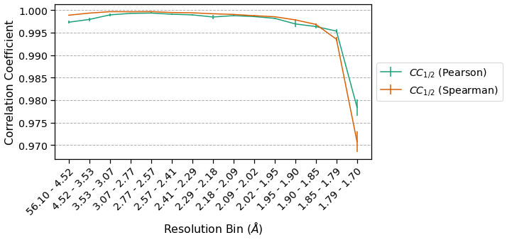
It is important to note the scale on the y-axis – this dataset is edge-limited, and as such the \(CC_{1/2}\) is very high across all resolution bins. The Spearman CC appears higher across all resolution bins except at high resolution, and overall has a lower standard deviation among samples. This is consistent with our expectation that Spearman CCs are a more robust estimator of correlation than Pearson CCs.

Let’s now repeat this for the anomalous data, computing \(CC_{anom}\):

merged["ANOM1"] = merged["I(+)1"] - merged["I(-)1"]
merged["ANOM2"] = merged["I(+)2"] - merged["I(-)2"]

# Similar to CChalf, but we will only look at acentric reflections
groupby2 = merged.acentrics.groupby(["sample", "bin"])[["ANOM1", "ANOM2"]]
pearson2 = groupby2.corr(method="pearson").unstack().loc[:, ("ANOM1", "ANOM2")]
pearson2.name = "Pearson"
spearman2 = groupby2.corr(method="spearman").unstack().loc[:, ("ANOM1", "ANOM2")]
spearman2.name = "Spearman"
results2 = rs.concat([pearson2, spearman2], axis=1)
results2 = results2.groupby("bin").agg(["mean", "std"])

results2.head()

	Pearson		Spearman
	mean	std	mean	std
bin
0	0.422196	0.037998	0.497923	0.029704
1	0.233349	0.061975	0.328263	0.023917
2	0.357182	0.051746	0.444657	0.029250
3	0.484710	0.045454	0.543314	0.031731
4	0.579058	0.023952	0.611739	0.020141

plt.figure(figsize=(8, 4))
plt.errorbar(results2.index, results2[("Pearson", "mean")],
             yerr=results2[("Pearson", "std")],
             color="#1b9e77",
             label=r"$CC_{anom}$ (Pearson)")
plt.errorbar(results2.index, results2[("Spearman", "mean")],
             yerr=results2[("Spearman", "std")],
             color="#d95f02",
             label=r"$CC_{anom}$ (Spearman)")
plt.xticks(results2.index, labels, rotation=45, ha='right', rotation_mode='anchor')
plt.ylabel("Correlation Coefficient")
plt.xlabel(r"Resolution Bin ($\AA$)")
plt.legend(loc='center left', bbox_to_anchor=(1, 0.5))
plt.grid(axis="y", linestyle='--')
plt.show()

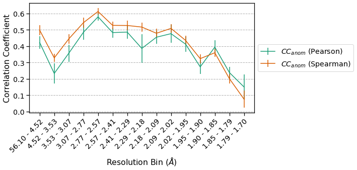
There is significant anomalous signal across all but the highest resolution bins. The Spearman CCs have smaller error bars than the corresponding Pearson CCs and the Spearman CCs are also higher in most bins. These differences highlight the influence of outlier measurements on the different correlation coefficients.

---

Summary

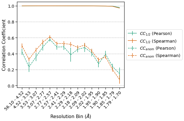
We have used reciprocalspaceship to merge a dataset using inverse-variance weights. As part of this analysis, we performed repeated 2-fold cross-validation to compute Pearson and Spearman correlation coefficients and associated uncertainties. This relatively simple procedure to obtain uncertainty estimates for correlation coefficients is seldom done when analyzing merging quality. However, we can see that the standard deviation for computed correlation coefficients can be nearly \(\pm0.1\) for quantities such as \(CC_{anom}\). This is worth keeping in mind when analyzing SAD experiments because this dataset is very high quality (edge-limited) when one considers the \(CC_{1/2}\). Putting these two correlation coefficients on the same axes emphasizes this point:

plt.figure(figsize=(9, 6))
plt.errorbar(results1.index, results1[("Pearson", "mean")],
             yerr=results1[("Pearson", "std")],
             color='#1b9e77',
             label=r"$CC_{1/2}$ (Pearson)")
plt.errorbar(results1.index, results1[("Spearman", "mean")],
             yerr=results1[("Spearman", "std")],
             color='#d95f02',
             label=r"$CC_{1/2}$ (Spearman)")
plt.errorbar(results2.index, results2[("Pearson", "mean")],
             yerr=results2[("Pearson", "std")],
             color='#1b9e77',
             linestyle="--",
             label=r"$CC_{anom}$ (Pearson)")
plt.errorbar(results2.index, results2[("Spearman", "mean")],
             yerr=results2[("Spearman", "std")],
             color='#d95f02',
             linestyle="--",
             label=r"$CC_{anom}$ (Spearman)")
plt.xticks(results1.index, labels, rotation=45, ha='right', rotation_mode='anchor')
plt.ylabel(r"Correlation Coefficient")
plt.xlabel(r"Resolution Bin ($\AA$)")
plt.legend(loc='center left', bbox_to_anchor=(1, 0.5))
plt.grid(axis="y", linestyle='--')
plt.tight_layout()

Even a simple change to the procedure for computing merging statistics, such as substituting a Spearman correlation coefficient for a Pearson one, can alter the apparent quality of a dataset. By lowering the barrier to implementing new analyses, we hope that reciprocalspaceship can encourage the development of more robust indicators of crystallographic data quality.