21 Mar 2025
Deep learning for Electron Density Map Sharpening
Project Report of using diffusion model for super-resolution
Daisy Liu
Project Problem Statement and Motivation
What are Electron Density Maps?
X-ray crystallography and Cryo-electron microscopy are important techniques to determine atomic-level information of biological molecules such as proteins and DNA. When a beam of X-rays is directed at the crystal, it is scattered by atoms in the lattice, producing a diffraction pattern of spots reflecting the geometry of the crystal. The brightness of these spots contains information about the structure of the molecule. This diffraction patten can then be used to generate electron density maps which encode this structural information and are widely used in many fields including structural biology, biochemistry, and biophysics.
Why is Super-Resolution Needed?
Electron density maps often have low resolutions, making it difficult to extract information of fine structural details.
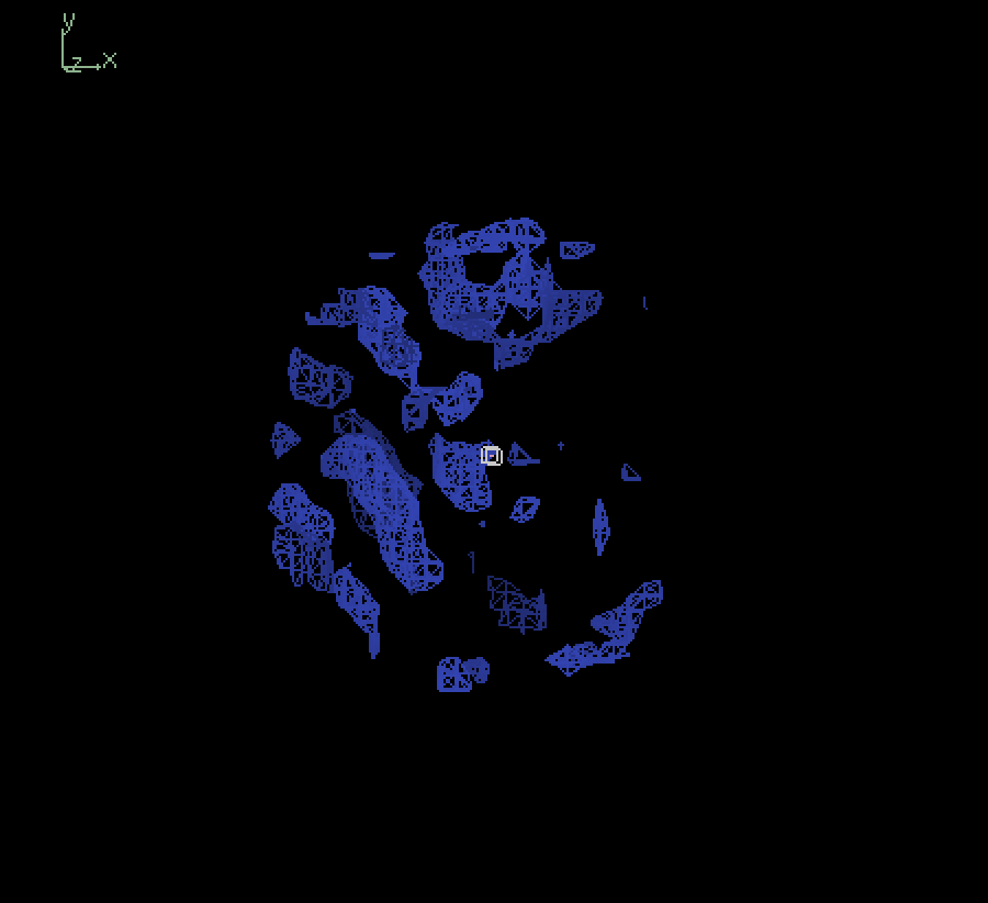
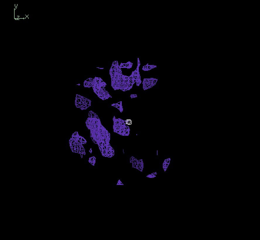
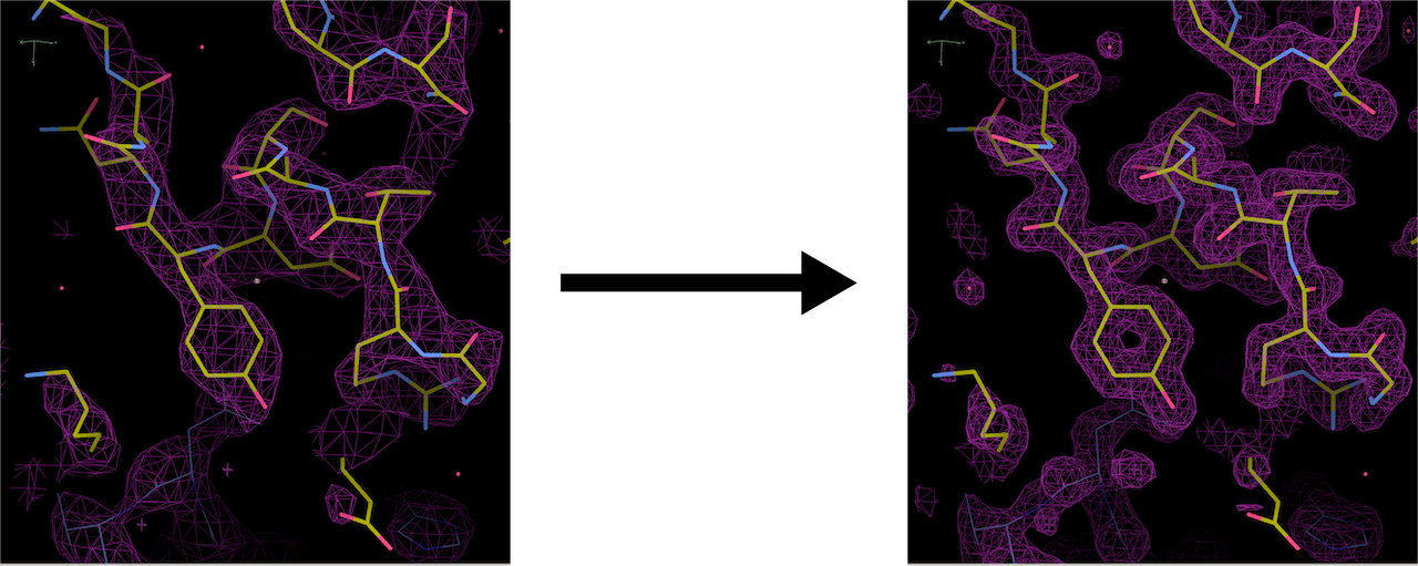 Figure 1: Example of an electron density map.
Currently, it takes a significant amount of time for experts to interpret an atomic model from X-ray or electron microscopy data, and structural biology experiments are often expensive. One major cost associated with such experiments is the time spent manually fitting atomic coordinates into electron density maps. An effective map sharpening model has the potential to make maps easier to interpret thereby decreasing the amount of expert time spent and reducing the cost. Such a model may also be used for new applications like interpolating between observed experimental results such as time points in a chemical reaction.
Why Generative Models?
A major challenge in super-resolution is that one lower resolution input map is compatible with multiple higher resolution ones. This issue remains unaddressed by much of the existing research, which largely focuses on non-generative approaches. This motivates us to consider generative approaches in our project to address this one-to-many mapping issue.
Model Framework and Architecture
Overall, we considered three models: an initial baseline taken from existing research and two generative models - a variational autoencoder (VAE) and a denoising diffusion model which are becoming increasingly popular in X-ray crystallography. Here, we focus on the diffusion model used in the project.
Conditional Denoising Diffusion Model
We used a conditional denoising diffusion model originally proposed in Ho et al., 2020. The model is designed to enhance electron density maps by progressively refining noisy inputs into sharper, high-resolution representations. Unlike single-step generative models, diffusion models learn a structured noise-removal process over a large amount of timesteps and is expected to have better performance because of this gradual denoisng process.
Following the DDPM framework, we first define a forward diffusion process to gradually add Gaussian noise \(\epsilon \sim \mathcal{N}(0,\ \mathbf{I})\) into a higher-resolution map \(y_0\). Using the Markov property and re-parameterization tricks, the distribution at an arbitrary time step can be calculated as:
\[q(\mathbf{y}_t \mid \mathbf{y}_0) = \mathcal{N}(\mathbf{y}_t ; \sqrt{\bar{\alpha}_t} \mathbf{y}_0, (1 - \bar{\alpha}_t) \mathbf{I})\]This enables us to employ a random sampling of time step \(t \in \{0, \dots, T\}\) in the forward process.
Training of the neural network occurs in the reverse process. Starting from random noise, the model learns a parametric approximation to the sample distributions, and iteratively refines the image to obtain a high-resolution target map.
In essence, the diffusion model first gradually adds noise in the forward pass, and then gradually learns to “undo” the noise, recovering the ground truth map. Figure 2 below gives an illustration of this process.
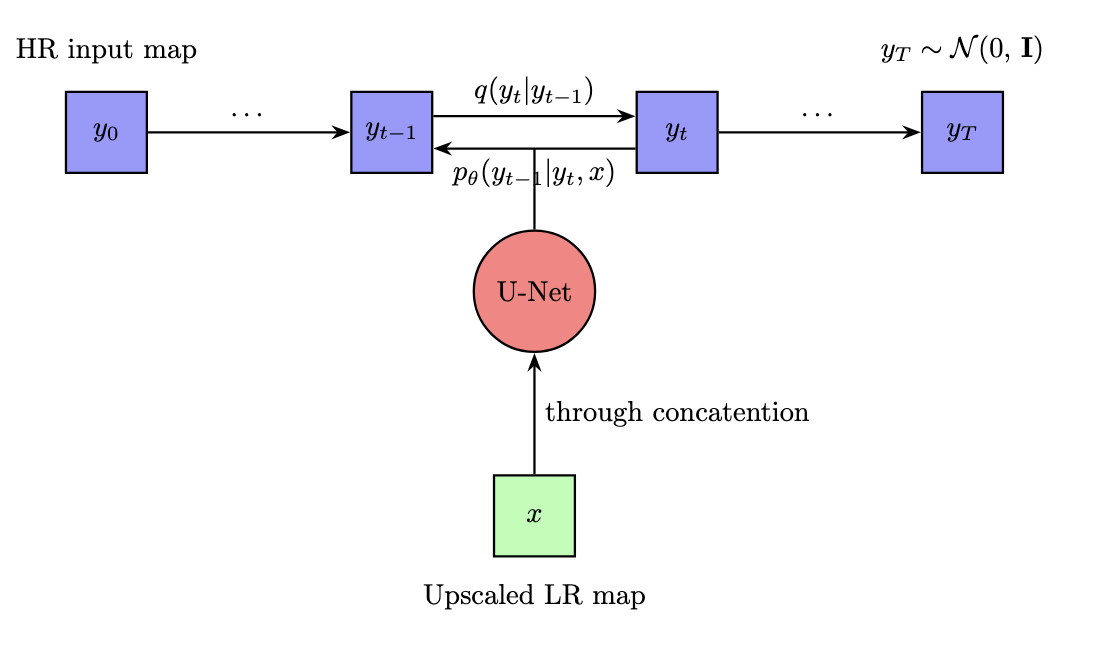 Figure 2: Framework for Diffusion Model.
Algorithms
To formalize the process described above, we show some summaries of the training and sampling algorithms we used:
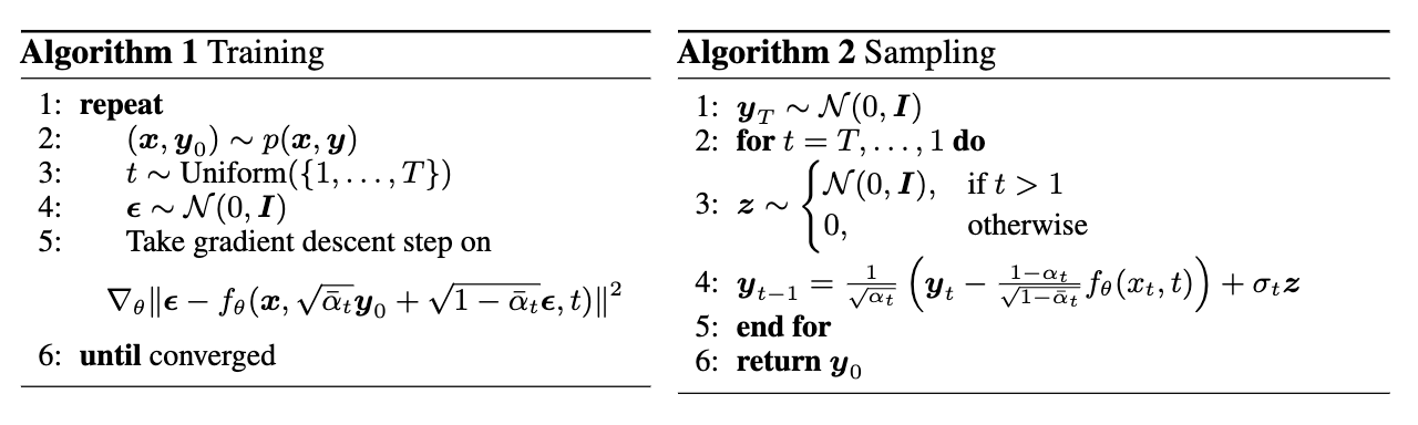 Figure 3: Diffusion Model Algorithms.
In the training algorithm, following the same algebraic derivations in the original DDPM paper, the training objective function can be simplified to
\[{\lVert \boldsymbol{f}_\theta(x, y_t, t)-\boldsymbol{\epsilon} \rVert}^2\]where \(f_\theta\) is our denoising function conditional on an upscaled input \(x\) for more control of the output. Hence, the model is trained to predict the noise produced, which can then be subtracted from the \(y_t\) to obtain a denoised map \(y_{t-1}\). We use a typical DDPM U-Net adapted for 3-dimensional inputs as \(f_\theta\).
Current Progress and Challenges
Training Progress
So far, we have successfully implemented the diffusion model and begun training. Initially, we tested a smaller version of the model using 2,000 samples and 200 timesteps over 50 epochs. This training completed smoothly in about two hours. We then moved on to training the full model with 20,000 samples and 1,000 timesteps— a setting recommended in the literature for optimal performance. However, these runs stalled after just a few epochs, likely due to the high memory demands of the 3D diffusion process, particularly with the self-attention blocks used in the denoising step.
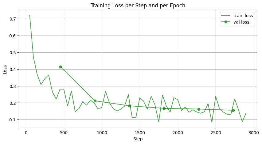
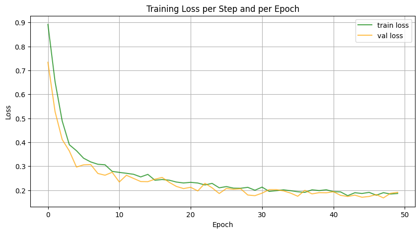 Figure 4: Learning Curves of Model.
Figure 4 above displays the learning curves from two representative training runs: one for the smaller model (right) and one for the full-sized model (left). In the second plot, both training and validation loss start high and decrease smoothly over epochs, showing effective learning. The validation loss follows the training loss closely, indicating that the model generalizes and there is little overfitting. In the first plot for the full model, losses are plotted against steps. Although training only reached epoch 4, the training loss drops rapidly to around 0.2, with some fluctuations. The validation loss follows a similar downward trend.
The rapid initial decrease in loss is a common characteristic of diffusion models. This behavior arises because diffusion models learn to reverse a well-defined noise process, where the early training stages focus on reconstructing coarse structural details from highly corrupted inputs. Since large-scale patterns are easier to recover than fine details, the model quickly improves in the first few epochs. As training progresses, the model shifts to learning finer details, causing a slower, more gradual improvement.
Training Challenges and Attempts
The greatest issue with the training process is memory usage. We were initally having CUDA out of memory issues constantly. Upon requesting more GPU and CPU memory for the training job, we found that training was often stuck in the initial epochs. To diagnose and fix these issues, we made several attempts, including reducing batch sizes, increasing num_workers in dataloaders for more parallelization, and adding logs to record timings and memory usage of each process.
The timing results within the diffusion model shows that setting new noise schedule and running each forward pass are fast, taking less than 0.001 sec on average becuase of the direct use of reparameterization. Each training step and loss computation takes ~0.05 sec, but there are outliers where steps take over a minute, mostly happening at the beginning of the process. These results are expected for a well-optimized diffusion model, with initial slow speed caused by CUDA initialization. Therefore, the training issues are unlikely due to model computations.
We then used psutil to log memory usage. The figure below shows the values recorded in a standard run for about 1 hr, where training starts at timestamp 13:22:38.
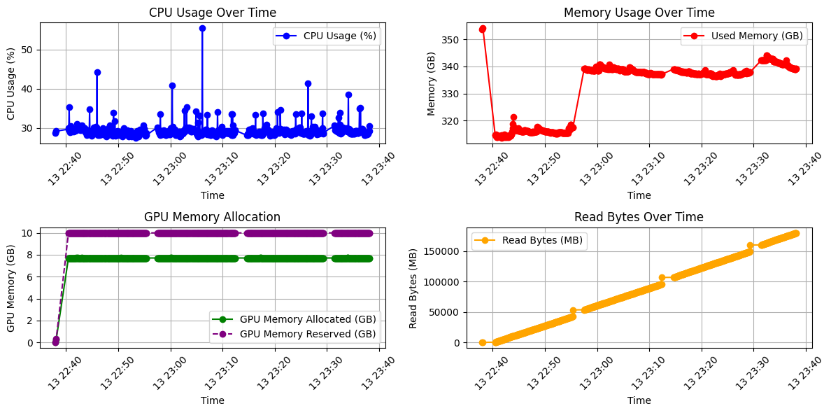 Figure 4: Memory Usage.
The figures indicate that there is no evidence of a CPU bottleneck, and GPU memory allocation remains sufficient throughout the process. However, the “Read Bytes” values increase linearly and steadily, reaching extremely high levels (~180GB) just before training stalls. This result, combined with the observation that increasing num_workers and reducing batch size had minimal impact, suggests a likely I/O bottleneck. In light of these findings, we are now transitioning to training with local scratch storage. This is a suggested approach to mitigate the impact of slow network access when handling large datasets. Currently, we have copied training data into local scratch, but are still working on setting up the data loading pipeline from scratch.
Inference
Inference of the diffusion model also presented challenges, as we initially observed complete misalignments between the input and output electron density maps. Through experimentation, we found that normalizing the grids at each resolution step was crucial in mitigating these misalignments. Interestingly, this preprocessing step was not necessary for our other models, such as the baseline UNet and VAE. While min-max normalization (scaling pixel intensities between -1 and 1) is commonly suggested in the literature, we found that it did not improve results compared to the z-score normalization we are currently using.
Since our full-sized model was not trained extensively, we primarily tried inference using our smaller model. The figure below shows the input map and inference outputs for the molecule with pdb ID 12e8:
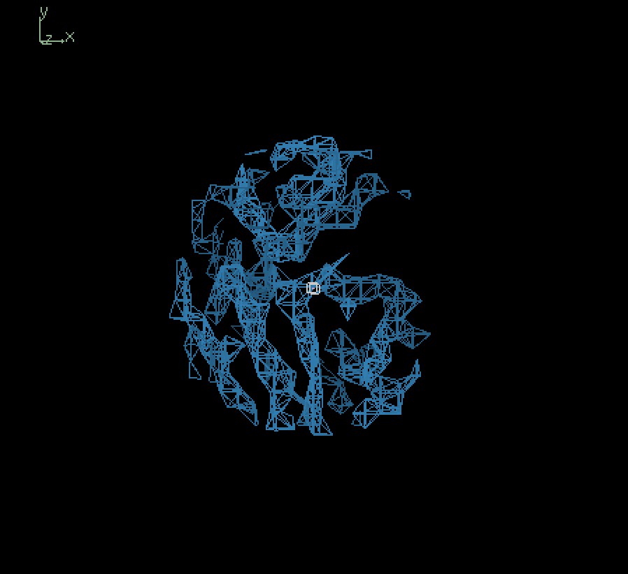 Input (4.0Å) |
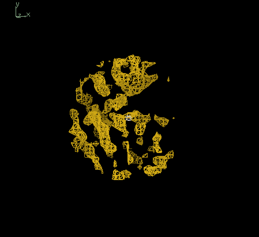 Output (4.0Å) |
 Output (3.0Å) |
 Output (2.0Å) |
The results show that although our model appears to be successfully capturing the coarse structural details, there are places of discontinuities and misalignment. To analyze the results quantitatively, we calculated the fourier shell correlation coefficient(FSC) values at different resolutions between the input 4.0Å map and output 4.0Å map, in which case the model is effectively trying to output a denoised version of the input, starting from pure gaussian noise at the last timestep. At low resolutions (>4.0Å), the FSC values exceeded the commonly used cutoff of 0.143 suggesting a degree of structural similarity. However, the relatively low correlation (~0.2 to 0.3) indicates that the model struggles to recover fine details. Therefore, its overall performance is limited, likely due to its small size and incomplete training. Moving forward, we plan to evaluate inference quality using a fully trained full-scale model, which should yield more reliable structural reconstructions.
Future Work
Our immediate next step is to continue troubleshooting and train the full-scale model extensively. To aid in debugging, we are implementing callbacks within the training script to run inference at regular intervals. By analyzing these results, we aim to gain a deeper understanding of the model’s behavior and potential failure modes.
While our current inference results produce meaningful electron density maps, we have observed that pixel intensity values exceed the expected range, indicating possible numerical instabilities. Addressing this issue will be a second focus moving forward. Additionally, we will perform hyperparameter tuning, particularly optimizing noise schedules and learning rates, to improve model stability and performance.
Beyond qualitative evaluation, we also plan to incorporate quantitative metrics such as PSNR and SSIM to assess model performance. In the long term, we aim to refine the model’s architecture and improve performance beyond the baseline DDPM.
References
Ho, J., Jain, A., & Abbeel, P. (2020). Denoising diffusion probabilistic models. Advances in Neural Information Processing Systems, 33, 6840–6851.
Saharia, C., Ho, J., Chan, W., Salimans, T., Fleet, D. J., & Norouzi, M. (2023). Image super-resolution via iterative refinement. IEEE Transactions on Pattern Analysis and Machine Intelligence, 45(5), 4713–4726.