31 Aug 2026

Are We Capturing the Ensemble?

What structural biology experiments preserve, blur, or discard about molecular distributions

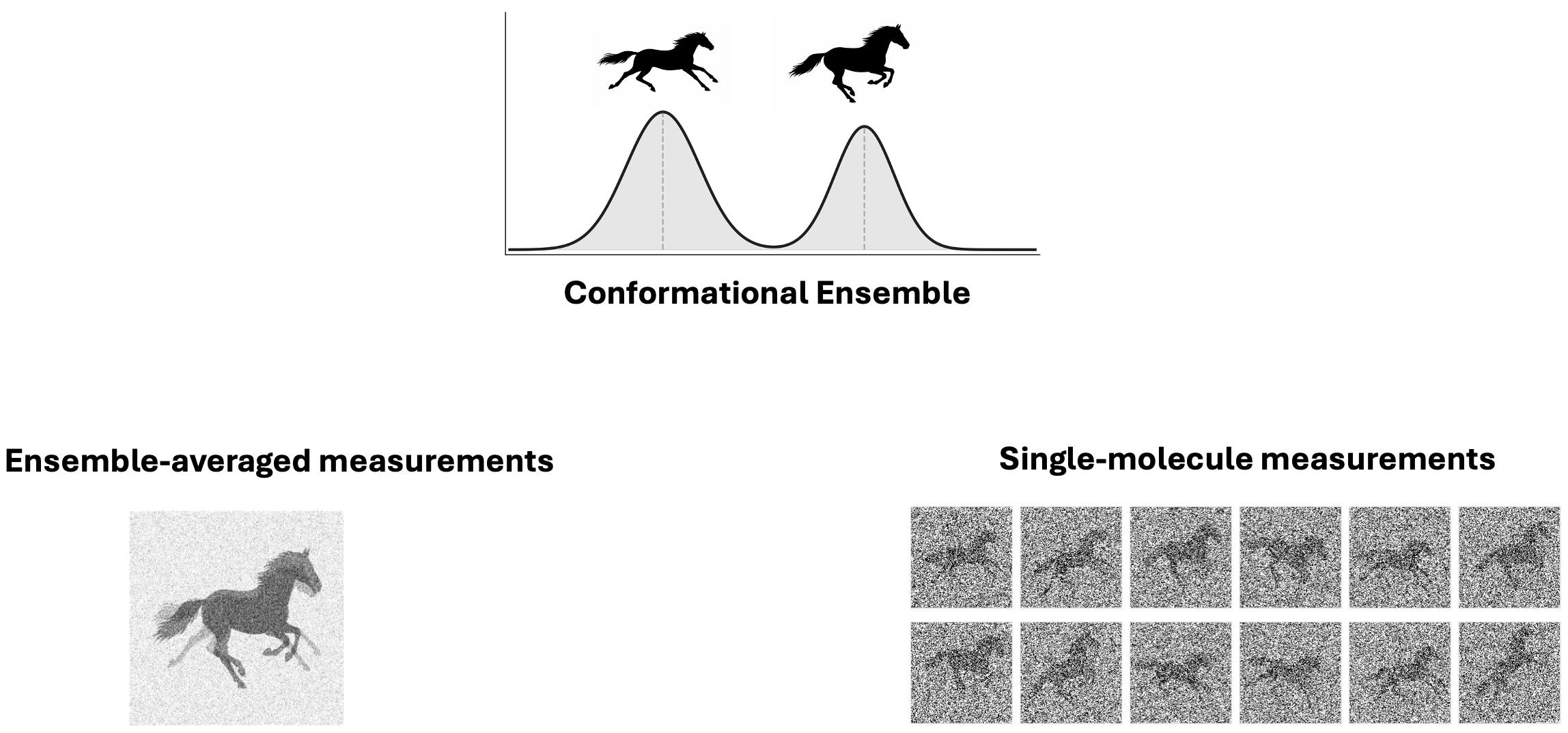Minhuan Li, F. Emil Thomasen, Pilar Cossio{minhuanli,fthomasen,pcossio}@flatironinstitute.org

Two ways an experiment can encode a conformational ensemble Two ways in which an experiment can encode a conformational ensemble. Ensemble-averaged measurements combine contributions from many molecules into each observable. In single-particle measurements, each observation arises from an individual molecule, and the ensemble is represented statistically across many observations.

Structural biology is increasingly being asked to answer questions about ensembles rather than single structures. But two opposite intuitions can lead us astray. In cryo-electron microscopy (cryo-EM), a fuzzy or weak region of a reconstructed map is sometimes treated as if it were direct evidence of an ensemble: blur becomes heterogeneity. In the other direction, an experiment such as X-ray diffraction may be dismissed as incapable of constraining an ensemble because its measurements average over many molecules.

These intuitions seem contradictory, but they make the same mistake. Both assume what an experiment can tell us about a molecular distribution from the appearance of its final representation, rather than from how the data were generated or processed. A blurred map is not itself an ensemble distribution. But neither does averaging an observable necessarily collapse a distribution to a single structure.

The more useful question is therefore not whether a dataset “contains an ensemble”. It is which differences between molecular distributions remain observable after measurement and subsequent data processing. Two distinct ensembles may produce measurably different signals, or they may become indistinguishable once projected through experimental noise, limited observables, nuisance variables, finite sampling, or data reduction.

To make this question precise, we first need to distinguish the distribution we ideally would like to learn from the one the experiment actually sees.

What distribution enters the experiment?

Before asking what information the measurement pipeline preserves, we should first be clear about what distribution is being measured. Let \(p_{\mathrm{target}}(x)\) denote the molecular distribution relevant to the scientific question, and \(p_{\mathrm{src}}(x)\) the source distribution actually present in the prepared sample when the measurement is made. We refer to \(p_{\mathrm{src}}\) as the molecular ensemble distribution—the distribution we can, in principle, attempt to measure and infer. Often we hope that \(p_{\mathrm{src}}\) faithfully represents \(p_{\mathrm{target}}\), but the two need not be identical.

The distinction is especially concrete in cryo-EM, where vitrification is itself a physical process acting on the ensemble. Recent work by Clark et al. examined how rapid cooling can perturb conformational populations and how equilibrium populations might subsequently be inferred from the vitrified ensemble [6]. More generally, temperature, chemical environment, sample preparation, and experimental timescales can all affect the relationship between the distribution of biological interest and the one presented to the instrument.

The possible difference between \(p_{\mathrm{target}}\) and \(p_{\mathrm{src}}\) is important, but it is not the problem we will pursue here. We will take the source distribution as the object presented to the experiment and ask what happens next:

\[p_{\mathrm{src}}\longrightarrow\text{measurements}\longrightarrow\text{processed data}.\]

Which distinctions within \(p_{\mathrm{src}}\) survive this chain?

How experiments constrain the source distribution

Different experiments encode \(p_{\mathrm{src}}\) in different ways. Broadly, there are two useful cases. In an ensemble-averaged measurement, each observable combines contributions from many molecules. In a single-molecule measurement, individual observations arise from individual molecules, and the distribution appears statistically across many observations. These are not rankings of how much “ensemble information” an experiment contains. They are different ways of constraining the same underlying distribution.

For an ensemble-average measurement, in its simplest form, the observable can be written as

\[\int m(x)\,p_{\mathrm{src}}(x)\,dx + \varepsilon,\]

where \(m(x)\) is the forward model for the observable and \(\varepsilon\) represents measurement uncertainty. The experiment doesn’t measure the observable for any individual molecule. Instead, it reports the expectation value of that observable over the source distribution.

Importantly, averaging in observable space is not the same as averaging in conformational space. Suppose two conformations, \(x_A\) and \(x_B\), occur with probabilities \(p_A\) and \(p_B\). The measured signal is \(p_A m(x_A)+p_B m(x_B)\) not, in general, \(m\left(p_A x_A+p_B x_B\right)\). This distinction matters. If the observable responds differently to the two conformations, their contributions can remain separately constrained even though the measurement averages over many molecules. X-ray diffraction intensities, for example, need not correspond to a fictitious structure halfway between two populated conformations. Spatially distinct states can leave distinct contributions to the measured density. “Averaged” therefore does not mean “only informative about an average structure.”

Single-particle experiments preserve a different kind of information. We can describe an individual observation as arising from a latent molecular state,

\[x_n \sim p_{\mathrm{src}}(x),\]

together with experimental nuisance variables \(z_n\), followed by a measurement process \(K\),

\[y_n \sim K(\cdot \mid x_n,z_n)\,.\]

In single-molecule FRET, time traces of the same molecule can reveal transitions between coarse conformational states. In single-particle cryo-EM, time is not preserved: each particle contributes a noisy projection of one molecular configuration, and the ensemble appears through variation across many different particles.

For independent observations, their marginal distribution is

\[\int K(y\mid x,z)\cdot\pi(z)\cdot p_{\mathrm{src}}(x)\,dz\,dx.\]

Because molecule-to-molecule variation has not been collapsed immediately into a small set of ensemble averages, such data can in principle retain rich information about heterogeneity. But molecule-resolved does not mean that the underlying distribution is directly observed. Noise, unknown nuisance variables, limited sampling, and the magnitude and diversity of conformational variation can make distinct molecular states difficult—or impossible—to distinguish.

The important point is therefore not that one class of experiment “measures ensembles” while the other does not. Both impose constraints on \(p_{\mathrm{src}}\), but they preserve different types and levels of distinctions within it.

A next key question is what happens in the downstream analysis: to what extent does subsequent data processing preserve the information encoded in \(p_{\mathrm{src}}\)?

How processing can wash out the source distribution

The physical measurement is not the end of the information chain. Raw observations are subsequently selected, transformed, clustered or averaged, into representations used for interpretation and inference. These operations may be essential for extracting useful signal, but they can also change which information about \(p_{\mathrm{src}}\) remains accessible downstream.

Cryo-EM provides a clear example. The standard reconstruction pipeline filters particles, estimates their poses, separates or models heterogeneity, and combines many observations into three-dimensional reconstructions. These steps are extraordinarily effective for recovering high-resolution structural detail. But particle filtering can remove observations, classification can partition continuous variation into discrete groups, and a consensus reconstruction can combine heterogeneous particles into a single representation. Information about the populations and variation present across the original particles may therefore no longer be recoverable from the reconstructed map alone.

Processing does not change the physical \(p_{\mathrm{src}}\) that generated the observations. But it changes what information about that distribution survives in the representation we choose to analyze. Ensemble information can therefore be lost at two stages: when the source distribution is converted into measurements, and again when those measurements are converted into processed data. Understanding what ensemble information is washed out in an experiment requires following that information through the entire pipeline.

The question of ensemble resolution

Just as spatial resolution asks when nearby features blur together, we can ask when two source distributions become indistinguishable after passing through the measurement and processing pipeline. We use ensemble resolution to refer to this question: which differences between molecular distributions remain distinguishable, given the uncertainty of the data and the transformations applied to them?

The analogy to spatial resolution is useful, but it only goes so far. Ensembles can differ in more than one way, so there is no reason to expect a single number to summarize their resolution. Two distributions might contain the same major conformations but assign them different populations; one might contain a rare state absent from the other; or they might show similar fluctuations individually but differ in how those motions are correlated. A dataset may distinguish one of these differences while being nearly blind to another. What can be resolved therefore depends not only on the experiment, but also on what aspect of the distribution we are asking it to distinguish.

Cryo-EM makes the distinction between spatial and ensemble resolution especially concrete. A reconstruction can gain spatial resolution while losing ensemble resolution. This is also why weak or fuzzy density should not, by itself, be interpreted as an ensemble. Such density can have many sources, including experimental uncertainty. But even if the blur genuinely comes from conformational heterogeneity, heterogeneity alone does not specify a distribution. The same diffuse density could arise from different sets of conformations, populations, or correlated motions across the particles.

In a more controlled inference setting, we are beginning to see how the question of ensemble resolution can be formalized. Ensemble reweighting, for example, starts from a specified set of candidate conformations and asks how experimental measurements constrain their populations. Once the possible states are fixed, one can ask more precisely which differences in population are supported by a given set of measurements and their uncertainties [7]. General ensemble inference is harder: both the conformations themselves and their probabilities may be unknown. How to characterize ensemble resolution in that setting remains a much broader open problem.

The takeaway

Before arguing for an ensemble-inference method, ask how the data were generated, what transformations they underwent, and which distinctions within the source distribution remain observable. An averaged measurement can still constrain multiple states; a molecule-resolved experiment does not make the ensemble directly visible; and a high-resolution reconstruction may preserve less population information than the observations from which it was built.

Thinking in terms of ensemble resolution shifts the question from whether an experiment “contains an ensemble” to a more useful one: what aspects of the molecular distribution can this dataset actually distinguish?

Thanks to T.J. Lane and Alisia Fadini for reading earlier drafts and for their thoughtful feedback.