03 Aug 2026

Are We Seeing the Ensemble?

How structural biology experiments preserve, blur, or lose molecular ensembles

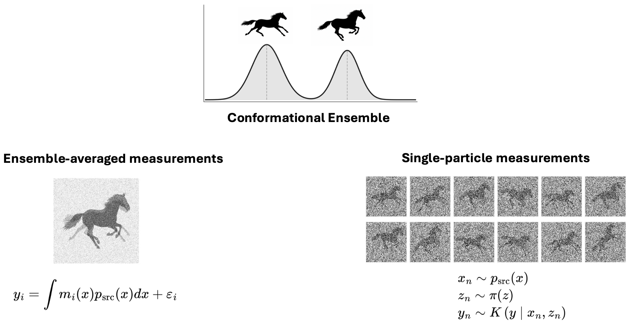Minhuan Li, F. Emil Thomasen, Pilar Cossio{minhuanli,fthomasen,pcossio}@flatironinstitute.org

Two ways an experiment can encode a conformational ensemble Two ways in which an experiment can encode a conformational ensemble. Ensemble-averaged measurements combine contributions from many molecules into each observable. In single-particle or single-molecule measurements, each observation arises from an individual molecule, and the ensemble is represented statistically across many observations.

Ensemble-inference approaches are rapidly becoming a research frontier across structural biology. But asking a biophysical experiment for a distribution is different from asking it for a structure. Before reaching for a better inference method, we first have to ask how the experiment encoded the ensemble and how much of that information survived measurement and processing. Different modalities answer this question differently: some measure noisy samples from the distribution, while others compress the ensemble into a set of averaged observables.

This distinction cuts across structural biology. Here we begin with cryo-electron microscopy (cryo-EM), where particle images and reconstructed maps provide two different observables of the same sample. Their contrast illustrates a broader principle that will apply across experimental modalities: the suitability of a target for ensemble inference depends not only on its structural detail, but also on how faithfully it retains information about the underlying distribution. To understand why, start with the object we are trying to recover.

Biomolecules as thermodynamic ensembles

Many structural models represent a biomolecule with a single set of coordinates. However, to perform their biological function, biomolecules populate a range of conformations: binding pockets must reshape to bind drugs, enzymes must deform to catalyze reactions, ion channels must transition between open and closed states to regulate ion flux, and viral spike proteins must undergo large-scale openings to infect host cells.

An ensemble is more than the observation that molecules move. It describes both which conformations are accessible and how frequently they occur. This information is captured by a probability distribution over molecular configurations, the thermodynamic ensemble. At temperature \(T\), the equilibrium ensemble follows Boltzmann’s distribution,

\[p_{\mathrm{th}}(x) = \frac{1}{Z}\exp\!\left(-\frac{E(x)}{k_B T}\right), \tag{1}\]

where \(x\) is a molecular conformation, \(E(x)\) is its potential energy, \(k_B\) is Boltzmann’s constant and \(Z\) is the partition function. Knowing \(p_{\mathrm{th}}(x)\) tells us which conformations are populated and with what probabilities, including rare or transition states. Together with an appropriate forward model, it would also allow us to predict equilibrium measurements.

A single deposited structure might be a useful summary of this landscape, but certain questions can only be addressed with the ensemble distribution: how populated is an alternative conformation, how often does a cryptic pocket open, which states are stabilized by a drug, and which motions disappear after a mutation? Once these are the questions — ones that bring us closer to understanding the biological role of a biomolecule — structure determination becomes ensemble inference.

But this ideal distribution might not be the one that enters the instrument. Experiments instead probe a source distribution, \(p_{\mathrm{src}}\), present in the prepared sample under the conditions of measurement. Sample preparation, temperature, chemical environment, and the conformational timescales of the molecule can all separate this distribution from the physiological ensemble we ultimately care about. This gap applies to every modality, not only to cryo-EM. Ensemble inference therefore has two layers: recovering \(p_{\mathrm{src}}\) from the data, and deciding how faithfully \(p_{\mathrm{src}}\) represents \(p_{\mathrm{th}}\). Here we focus on the first.

How experiments observe the source distribution

Once the immediate target is \(p_{\mathrm{src}}\), the next question is what kind of trace the experiment leaves behind. Broadly, there are two, as illustrated in the figure at the top of this post. Some experiments combine contributions from many molecules into ensemble-averaged observables. Others are molecule-resolved: individual observations arise from individual molecules, and the ensemble appears statistically across many observations.

For an ensemble-average measurement, the data take the form

\[y_i = \int m_i(x)\,p_{\mathrm{src}}(x)\,dx + \varepsilon_i, \tag{2}\]

where \(m_i(x)\) is the forward model for observable \(i\) and \(\varepsilon_i\) is measurement noise. The experiment does not hand us individual conformations; it hands us a weighted average of the observable over the source distribution. How much ensemble information survives depends on what was averaged, how many independent constraints remain, and at what spatial resolution they were measured.

Averaging an observable is not the same as measuring the average structure. For two conformations \(A\) and \(B\), with source probabilities \(p^A_{\mathrm{src}}\) and \(p^B_{\mathrm{src}}\), respectively, what is measured is \(p^A_{\mathrm{src}}\,m(x_A) + p^B_{\mathrm{src}}\,m(x_B)\), not \(m(p^A_{\mathrm{src}} x_A + p^B_{\mathrm{src}} x_B)\). When the observable is close to linear in structural space, two spatially separated conformations can leave two separable traces rather than one fictitious midpoint. Averaged data can still contain ensemble information; the question is how much of it remains distinguishable.

Single-molecule experiments come in more than one form. Some follow the same molecule over time. In single-molecule FRET, for example, a time trace may be divided into coarse conformational states and used to estimate transitions; under stationary conditions, the distribution of that model estimates their populations. Such trajectories contain kinetic information as well as population information.

Cryo-EM preserves molecular individuality without preserving time. Each particle contributes a single noisy projection of one conformation, so the ensemble must be inferred from variation across many images rather than from transitions within a trajectory. Despite this difference, both experiments can be described as noisy observations of latent molecular states:

\[\begin{aligned} x_n &\sim p_{\mathrm{src}}(x), \\ z_n &\sim \pi(z), \\ y_n &\sim K(\,\cdot\mid x_n, z_n), \end{aligned} \tag{3}\]

where \(x_n\) is the molecular state, \(z_n\) collects nuisance variables, and \(K\) is the measurement kernel relating a latent state to an observation. For a trajectory experiment, this is only the marginal observation model; a complete description must also specify how states evolve in time. In cryo-EM, the index \(n\) instead runs over different particles, while \(z_n\) includes projection direction, translation, and microscope effects.

For independent snapshots — or for the marginal observation at one time point — the distribution of observations is

\[q(y) = \iint K(y \mid x, z)\,\pi(z)\,p_{\mathrm{src}}(x)\,dz\,dx. \tag{4}\]

Unlike Equation (2), this distribution retains molecule-to-molecule variation rather than reducing it immediately to selected averages. Yet recovering \(p_{\mathrm{src}}\) from \(q(y)\) remains an inverse problem. In cryo-EM, low contrast, unknown poses, microscope effects, and the high dimensionality of conformational variation can make that problem extremely difficult. Molecule-resolved does not mean easily recoverable, just as ensemble-averaged does not mean devoid of ensemble information. The two measurement routes therefore lose information differently. To compare them, we need to ask how different two source distributions must be before an experiment can distinguish them.

Ensemble resolution

We call this limit ensemble resolution. Just as spatial resolution asks when nearby features blur together, ensemble resolution asks when distinct source distributions become experimentally indistinguishable. More precisely, two distributions cannot be distinguished when, after passing through the measurement process, they produce observables that agree within the uncertainty of the data.

An experiment can therefore contain ensemble information and still have low ensemble resolution. It may distinguish open from closed but not resolve a continuum between them, detect a rare state but not determine its occupancy, or report a broad fluctuation without identifying the correlated motions that produced it. For averaged measurements, the limit is set by the number and spatial specificity of the independent constraints. For molecule-resolved measurements, it is set by how well different latent states remain distinguishable through noise, nuisance variables, finite sampling, and the inference model. In cryo-EM, this criterion exposes a second distinction: particle images and reconstructed maps sit at different stages of information loss.

Cryo-EM: two targets, structure or ensemble?

The crucial change occurs during reconstruction. Particle images that began as separate molecular observations are picked, curated, aligned, classified, masked, and averaged into a three-dimensional map. This processing is essential for high-resolution structure determination, but it also changes the inferential target.

A reconstructed map can be an excellent structural target. It may define a selected conformational state with impressive detail, and local heterogeneity can still appear as weak or diffuse density. But the map is not itself a molecule-resolved sample from \(p_{\mathrm{src}}\). It is a derived estimate conditioned on which particles were selected, how they were aligned and classified, and what priors entered the reconstruction. If a rare state was removed upstream, or continuous variation was forced into a small number of classes, no analysis of the resulting map can restore that lost population information.

For questions about the distribution represented by the collected particles, particle-level data are therefore the more natural starting point. They retain the variation across individual observations before it is collapsed into a consensus reconstruction. This does not make image-level ensemble inference easy: an algorithm must separate conformational variation from pose, microscope effects, noise, and finite sampling, often through a low-dimensional representation of molecular motion.

Cryo-EM therefore makes the central diagnostic concrete: before asking whether an inference method is powerful enough, ask whether its target still contains the distributional information of interest. Consensus maps are appropriate targets when the goal is a detailed structure. When the goal is to infer the distribution represented by the collected particles, however, a consensus map alone is not enough; inference should begin from particle-level data. In future pieces, we will apply the same framework to other modalities: what did the experiment preserve, what did it compress, and what did the analysis pipeline discard?

Are We Seeing the Ensemble?

How structural biology experiments preserve, blur, or lose molecular ensembles

Biomolecules as thermodynamic ensembles

How experiments observe the source distribution

Ensemble resolution

Cryo-EM: two targets, structure or ensemble?

Further reading