
Serial Pink-Beam Laue Processing of DHFR Data
This tutorial walks through processing polychromatic (“pink-beam”)
diffraction images as serial stills with laue-dials. In serial
crystallography every image comes from a different crystal, or from the
same crystal at an unknown orientation, so nothing can be assumed about
how one image relates to the next. Each image is therefore indexed on
its own with the pink-beam indexer built into DIALS (pinkIndexer),
and only then handed to the polychromatic laue-dials pipeline for
wavelength assignment, geometry refinement, prediction, and integration.
The data set is the E. coli dihydrofolate reductase (DHFR) Laue data
set that ships with the laue-dials examples. It was recorded on a
Rayonix MX340-HS detector with a 200 mm crystal-to-detector distance and
a spectrum peaking near 1.04 Å. The images were actually collected as a
rotation series with one degree between frames, but here we deliberately
ignore the goniometer and treat every frame as an independent still.
That makes this data set a convenient stand-in for a true serial
experiment: it exercises exactly the same code path, while still
allowing you to check the results against the rotation-series tutorial
if you wish.
This tutorial processes the complete 179-image data set. At the end
of processing we will have an integrated .mtz file that can be
scaled and merged with
`careless <https://github.com/rs-station/careless>`__.
Installation
The easiest way to install laue-dials and its dependencies is using
Anaconda
(or its lighter-weight cousins Miniforge/Micromamba). First update
conda and install the libmamba solver, which makes environment
creation much faster:
conda update -n base conda
conda install -n base conda-libmamba-solver
conda config --set solver libmamba
Then create and activate an environment for the install:
conda create --name laue-dials
conda activate laue-dials
Now install the main dependency, DIALS,
and then laue-dials itself with pip:
conda install -c conda-forge dials
pip install laue-dials
All other dependencies (including reciprocalspaceship, which writes
the final .mtz file) are installed automatically. Reopen this
notebook with the environment activated when you are ready.
Documentation for laue-dials can be found
here, and
entering any laue.* command with no arguments on the command line
prints a help page. This tutorial was run with DIALS 3.29 and laue-dials
0.5.1.
Introduction
The DHFR data set is available on
Zenodo. It contains 179 MCCD
images named e080_001.mccd through e080_179.mccd, plus a
pixels.mask file that blanks out the beamstop shadow and a few dead
regions of the detector.
This tutorial processes all 179 images. Every program in the pipeline
below takes an nproc (or N) argument to parallelize across
images, and nothing in the pipeline depends on how many images you give
it, so the same commands work unchanged on a subset or on a much larger
collection.
Copy (or symlink) all of the images into a directory called data
next to this notebook, and put pixels.mask in the working directory:
data/e080_001.mccd
data/e080_002.mccd
...
data/e080_179.mccd
pixels.mask
All of the commands in this tutorial are also collected in
serial_pipeline.sh, which you can run in
one go once you are comfortable with the individual steps. We use
N=12 throughout; adjust it to match the number of cores available on
your machine.
Importing Data
dials.import reads the images and their headers and writes an
experiment list (imported.expt) describing the beam, detector, and
(for rotation data) goniometer and scan. For MCCD images from this
beamline the header does not contain everything DIALS needs, so we
supply the missing pieces on the command line:
geometry.beam.wavelength=1.04— the peak wavelength of the spectrum. This is a placeholder used by the monochromatic algorithms; the polychromatic steps will assign a wavelength to every reflection individually.geometry.detector.panel.pixel=0.08854,0.08854— the pixel size in mm.geometry.scan.oscillation=0,1andgeometry.goniometer.axes=0,1,0— a nominal scan and rotation axis, needed only so that the format reader is happy. They are discarded in the next line.convert_sequences_to_stills=True— this is the key option for serial data. It tells DIALS to forget the scan and goniometer and to treat every image as an independent still experiment, which is what we want for a serial data set.lookup.mask=pixels.mask— the pixel mask. Applying it at import means it is stored in the experiment list and inherited by every later step.
dials.import geometry.scan.oscillation=0,1 \
    geometry.goniometer.axes=0,1,0 \
    convert_sequences_to_stills=True \
    geometry.beam.wavelength=1.04 \
    geometry.detector.panel.pixel=0.08854,0.08854 \
    lookup.mask=pixels.mask \
    input.template=$(pwd)/data/e080_###.mccd
The import summary at the end of the output should report
num stills: 179 and no sweeps. If you see a sweep instead,
convert_sequences_to_stills did not take effect and the later
stills-specific options will fail.
A quick way to check that the geometry is sensible is dials.show:
dials.show imported.expt | head -n 40
Spot Finding
Spot finding is exactly the same as for rotation data: we look for
connected pixels that rise above the local background on every image. We
call laue.find_spots, a thin wrapper around dials.find_spots
(either can be used interchangeably). The important parameters are:
spotfinder.threshold.dispersion.gain=0.15— the effective detector gain used by the dispersion threshold. Lower values find more (and weaker) spots; too low and you start picking up noise. For this detector 0.15 gives a clean set of strong spots.spotfinder.filter.max_separation=10— the maximum distance in pixels between a spot’s centroid and its brightest pixel. This rejects streaky or overlapping blobs that would confuse indexing.output.shoeboxes=False— do not store the pixel data for every spot in the reflection file. It keepsstrong.reflsmall; the integrator does its own pixel extraction later.lookup.mask=pixels.mask— the mask again, so masked pixels never become spots.
N sets the number of parallel processes. Raise it on a machine with
more cores and memory.
N=12

laue.find_spots imported.expt \
    output.shoeboxes=False \
    spotfinder.mp.nproc=$N \
    spotfinder.threshold.dispersion.gain=0.15 \
    spotfinder.filter.max_separation=10 \
    lookup.mask=pixels.mask
The log ends with a histogram of spots per image. Across the 179 images, each yields between roughly 390 and 610 strong spots, for 85,428 in total, and the counts are consistent from image to image, which is a good sign that the threshold is neither too high nor too low.
Viewing Images
The best way to judge spot finding is to look at the spots on the raw image. DIALS ships an interactive viewer for this:
dials.image_viewer imported.expt strong.refl
“Mark centers of mass” is ticked by default and draws the found spots as
red dots. If many obvious spots are not marked, lower the gain; if the
marks land on noise between the spots, raise it. The viewer also has a
tool for drawing new mask regions if you see scatter from the beamstop
or a bad panel that you want to exclude. We also pass brightness=60
(equivalent to raising the “Brightness” slider in the settings panel) to
make the faint diffuse scatter around the streaks easier to see.
The screenshot below is exactly what dials.image_viewer shows for
the first image once spot finding has run — no extra plotting code
required.
dials.image_viewer imported.expt strong.refl brightness=60
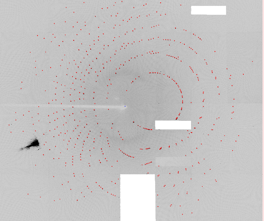
Spot finding results on the first image
The spots lie on the curved, streak-like loci typical of Laue diffraction: each streak is a row of reflections from one reciprocal-lattice line, spread out along the streak by the range of wavelengths in the beam. The masked beamstop arm and the dead rectangles show up as blank regions with no spots.
Indexing Each Still with pinkIndexer
Indexing is where serial data differ most from rotation data. With a
rotation series laue.index can use the known one-degree steps
between images to index every frame with a single crystal model. In a
serial experiment each image must be indexed on its own, and because the
beam is polychromatic we cannot use the usual monochromatic stills
indexers either: a reflection’s position on the detector no longer
determines its reciprocal-lattice vector until we know its wavelength.
DIALS includes the pinkIndexer algorithm (Gevorkov et al.,
2020) for exactly this
situation. Given the unit cell and an approximate wavelength range, it
searches for the crystal orientation that places the most observed spots
on lattice points for some wavelength inside the bandwidth. It is
selected in laue.index with
indexer.indexing.method=pink_indexer.
laue.index wraps dials.index; every dials.index parameter is
available under the indexer. prefix. The command below is long, so
here is what each group of parameters does:
Pink indexer parameters (indexer.indexing.pink_indexer.*)
wavelength=1.1andpercent_bandwidth=15define the wavelength window the indexer considers: 1.1 Å ± 7.5 %, i.e. roughly 1.02–1.18 Å. The window should cover the bulk of your spectrum. Note that it need not be centred on the placeholder wavelength given todials.import.max_refls=50— index using the 50 strongest spots on each image. More spots make the orientation search slower without much benefit.rotogram_grid_points=360andvoxel_grid_points=250control how finely orientation space is sampled. Finer grids give more precise starting orientations but need proportionally more memory per process (360 rotogram points needs a few GB per process on this data set) — raiseNand this grid together only as far as your machine’s memory allows.min_lattices=20— ask the indexer to generate up to 20 candidate lattices per image rather than stopping at the first few, so the stills indexer has more alternatives to choose between before picking a winner. In recent DIALS versions this option is deprecated in favour oftarget_lattices, which works the same way. Together, a fine rotogram grid and a generous lattice budget are what make pinkIndexer reliable on this data set: with a coarser grid (180 points) and fewer candidates (5) we found a noticeably larger fraction of images converged to the wrong lattice, visible later as outliers in the per-image RMSD after refinement.
Known symmetry (indexer.indexing.known_symmetry.*)
The space group (19, P2₁2₁2₁) and unit cell of DHFR. pinkIndexer requires a unit cell; it cannot determine one ab initio. If your cell is only approximately known, increase
percent_bandwidth, which also absorbs uncertainty in the cell lengths.
Stills indexing parameters (indexer.indexing.stills.* and
friends)
refinement_protocol.mode=None— do not refine the crystal model insidedials.index. Monochromatic refinement of polychromatic data would pull the model towards a compromise wavelength; we leave refinement to the polychromatic steps below.stills.refine_all_candidates=True,stills.rmsd_min_px=20, andstills.ewald_proximal_volume_max=0.03— every candidate lattice is scored with a quick stills refinement and the best one is kept. The thresholds are generous because, under the single-wavelength assumption, most reflections will not sit exactly on the Ewald sphere.joint_indexing=False— index every image independently. This is what makes the run “serial”: no information is shared between images.refinement.reflections.outlier.algorithm=None,parameterisation.auto_reduction.action=fix, andparameterisation.scan_varying=False— settings for the candidate refinement that avoid rejecting reflections or failing on stills with few spots.
Output
laue_output.index_only=True— skip the scan-varying refinement thatlaue.indexnormally runs after indexing. That refinement is meaningful only for rotation data. The indexed stills are written directly tomonochromatic.exptandmonochromatic.refl.
N=12

laue.index imported.expt strong.refl \
    indexer.indexing.nproc=$N \
    indexer.indexing.method="pink_indexer" \
    indexer.indexing.pink_indexer.wavelength=1.1 \
    indexer.indexing.pink_indexer.percent_bandwidth=15 \
    indexer.indexing.pink_indexer.max_refls=50 \
    indexer.indexing.pink_indexer.min_lattices=20 \
    indexer.indexing.pink_indexer.rotogram_grid_points=360 \
    indexer.indexing.pink_indexer.voxel_grid_points=250 \
    indexer.indexing.known_symmetry.space_group=19 \
    indexer.indexing.known_symmetry.unit_cell=34.297,45.552,99.035,90,90,90 \
    indexer.indexing.refinement_protocol.mode=None \
    indexer.indexing.stills.ewald_proximal_volume_max=0.03 \
    indexer.indexing.stills.rmsd_min_px=20 \
    indexer.indexing.stills.refine_all_candidates=True \
    indexer.indexing.joint_indexing=False \
    indexer.refinement.reflections.outlier.algorithm=None \
    indexer.refinement.parameterisation.auto_reduction.action=fix \
    indexer.refinement.parameterisation.scan_varying=False \
    laue_output.index_only=True
The log is long because the stills indexer reports a refinement for
every candidate lattice on every image. Look for the
Indexing imageset id banners to follow progress from image to image,
and for n_indexed in the summary after each one. Indexing all 179
images with N=12 took about seven minutes on the machine this
tutorial was run on.
Let us look at what came out. monochromatic.expt now contains 179
crystal models, one per image, and monochromatic.refl has the strong
spots with Miller indices assigned where the indexer could do so.
import numpy as np
from dials.array_family import flex
from dxtbx.model.experiment_list import ExperimentListFactory

mono_expts = ExperimentListFactory.from_json_file("monochromatic.expt", check_format=False)
mono = flex.reflection_table.from_file("monochromatic.refl")
strong = flex.reflection_table.from_file("strong.refl")

n = len(mono_expts)
per_strong = np.array([(strong["id"] == i).count(True) for i in range(n)])
per_indexed = np.array([(mono["id"] == i).count(True) for i in range(n)])
fractions = per_indexed / per_strong

cells_arr = np.array([e.crystal.get_unit_cell().parameters() for e in mono_expts])

print(f"Images indexed: {n}")
print(f"Strong spots: {per_strong.sum()}; indexed (monochromatic): {per_indexed.sum()}")
print(f"Fraction indexed: mean {fractions.mean():.2f}, "
      f"range {fractions.min():.2f}-{fractions.max():.2f}")
print("Mean unit cell (monochromatic): "
      + ", ".join(f"{v:.2f}" for v in cells_arr.mean(axis=0)))
print("Unit cell std dev: "
      + ", ".join(f"{v:.2f}" for v in cells_arr.std(axis=0)))
metric |
value |
|---|---|
images indexed |
179 |
strong spots |
85,428 |
indexed (monochromatic) |
32,817 |
fraction indexed, mean |
0.38 |
fraction indexed, range |
0.12 – 0.51 |
mean unit cell (Å) |
a = 34.19, b = 45.38, c = 98.96 |
unit cell std dev (Å) |
a = 0.08, b = 0.19, c = 0.28 |
Two things stand out, and both are expected:
Only about 38 % of the strong spots are indexed on average (ranging from 12 % to 51 % image-to-image). The stills indexer still assigns Miller indices using a single wavelength (1.04 Å), and only reflections whose true wavelength happens to be close to it satisfy the Ewald condition within the tolerance. The remaining spots are real, and
laue.optimize_indexingwill recover most of them in the next section.The unit cells are slightly off and scattered. Cell lengths from a monochromatic treatment of pink-beam data scale with the assumed wavelength, so
bin particular wanders by almost an Ångstrom from image to image. This does not matter here: the orientation is what we need from this step, and the cell will be reset and refined later.
The screenshot below shows the first image again, this time with only
the indexed subset of spots drawn (we pass show_indexed=True,
equivalent to ticking “Indexed” in the viewer’s reflection settings
panel). Compare it to the spot-finding screenshot above: indexed spots
cluster at particular positions along each streak — those are the
reflections whose wavelength happens to be near 1.04 Å — while their
neighbours along the same streak are left unindexed.
dials.image_viewer monochromatic.expt monochromatic.refl brightness=60 show_indexed=True
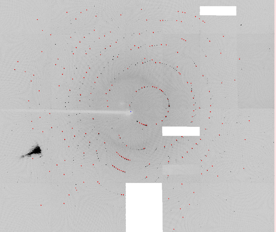
Indexed spots after monochromatic indexing
If indexing fails on some images (the log will say so and those images
are dropped from monochromatic.expt), the usual remedies are:
widen
percent_bandwidthso the wavelength window covers more of the spectrum;raise
max_reflsif the image has few strong spots, or lower the spot-finding gain to find more of them;check with
dials.image_viewerthat the beam centre and detector distance are right, since pinkIndexer is sensitive to both.
Note: with rotation data you would now run
laue.sequence_to_stills to split the scan into stills. Serial data
are already stills, so that step is not needed here.
Polychromatic Analysis
From here on the pipeline is the same as for rotation Laue data. Four
programs in laue-dials turn the monochromatic starting point into a
polychromatic model of each image:
laue.optimize_indexingassigns a wavelength to every reflection and refines the crystal orientation jointly, re-indexing the spots that the monochromatic step could not.laue.refineis a polychromatic wrapper fordials.refinethat refines the full experimental geometry against the wavelength-assigned reflections.laue.predictuses the refined geometry to predict the position and wavelength of every reflection that can appear on the detector, strong or weak.laue.integratefits spot profiles at the predicted positions and writes the integrated intensities to an.mtzfile.
Optimizing the Indexing Solution
laue.optimize_indexing takes the wavelength limits of the spectrum
(lam_min, lam_max) and a resolution limit (d_min) and, for
each image, alternates between assigning each spot the Miller index and
wavelength that best explain its position and rotating the crystal to
reduce the residuals. Serial-specific choices in this command:
geometry.unit_cell=...resets every crystal to the known DHFR cell before optimization. This removes the wavelength-dependent cell scaling we saw in the previous section. For rotation data one would usually let the cell fromlaue.indexstand.n_macrocycles=5— the number of assign/rotate cycles. Serial stills start from a rougher orientation than a scan-refined rotation series, so a couple of extra cycles (the default is 3) help them converge.By default
laue.optimize_indexingalso drops reflections that still cannot be indexed (keep_unindexed=False) and reflections whose assigned wavelength falls outside the stated spectrum (filter_spectrum=True), so they do not bias geometry refinement. Both are already the defaults, so we do not need to pass them explicitly.
N=12

laue.optimize_indexing monochromatic.expt monochromatic.refl \
    output.experiments="optimized.expt" \
    output.reflections="optimized.refl" \
    output.log="laue.optimize_indexing.log" \
    wavelengths.lam_min=0.97 \
    wavelengths.lam_max=1.20 \
    reciprocal_grid.d_min=1.4 \
    geometry.unit_cell=34.297,45.552,99.035,90,90,90 \
    n_macrocycles=5 \
    nproc=$N
from dials.array_family import flex

opt = flex.reflection_table.from_file("optimized.refl")
strong = flex.reflection_table.from_file("strong.refl")
wl = opt["wavelength"].as_numpy_array()

print(f"Indexed after optimization: {len(opt)} of {len(strong)} strong spots "
      f"({len(opt) / len(strong):.2f})")
print(f"Assigned wavelength range: {wl.min():.3f} - {wl.max():.3f} Angstrom")
metric |
value |
|---|---|
strong spots |
85,428 |
indexed, monochromatic |
32,817 (38 %) |
indexed, after optimization |
61,616 (72 %) |
assigned wavelength range |
0.970 – 1.200 Å |
Wavelength assignment very nearly doubles the number of indexed reflections, from about 38 % to 72 % of the 85,428 strong spots in this run (32,817 to 61,616 reflections).
The reflections that remain unindexed are mostly at the ends of the streaks, where the wavelength is outside the 0.97–1.20 Å window, or are harmonics and overlaps that no single Miller index can explain.
Refining the Geometry
laue.refine runs dials.refine with one beam per reflection, so
that the detector position, crystal orientation, and unit cell are
refined against the polychromatic observations. As with dials.refine
it detects and rejects centroid outliers before the final cycle; expect
to see a few percent of reflections flagged on each image.
N=12

laue.refine optimized.expt optimized.refl \
    output.experiments="poly_refined.expt" \
    output.reflections="poly_refined.refl" \
    output.log="laue.poly_refined.log" \
    nproc=$N
In this run, 178 of the 179 images successfully refine; one image had
too few reliable reflections for dials.refine to converge and is
dropped from poly_refined.expt. This is normal for a serial data set
— a real experiment would collect far more than 179 images precisely
because some fraction will fail at every stage.
Checking the Wavelength Spectrum
laue.plot_wavelengths histograms the wavelengths that were assigned
to the refined reflections. It should look like the spectrum of the
beam: for this undulator source a sharp peak near 1.04 Å with a long
tail to longer wavelengths. If the histogram is flat, or piles up at the
lam_min/lam_max limits, the wavelength assignment has gone wrong
and it is worth revisiting the indexing before going further.
laue.plot_wavelengths poly_refined.refl \
    refined_only=True \
    save=True \
    show=False \
    output=tutorial_images/wavelengths.png
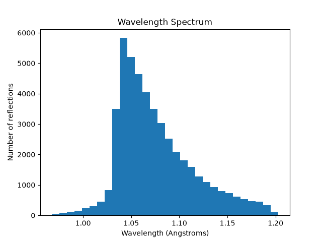
Histogram of assigned wavelengths
Checking the Residuals
laue.compute_rmsds reports, for each image, the root-mean-square
distance between observed and predicted spot centroids. Passing
refined_only=True restricts this to the reflections dials.refine
actually used (i.e. after its own outlier rejection), which gives a much
cleaner signal for spotting mis-indexed images than including every
reflection. An image with a much larger RMSD than its neighbours has
probably been mis-indexed.
laue.compute_rmsds poly_refined.expt poly_refined.refl \
    refined_only=True \
    show=False \
    save=True \
    output=tutorial_images/residuals.png \
    csv=rmsds.csv
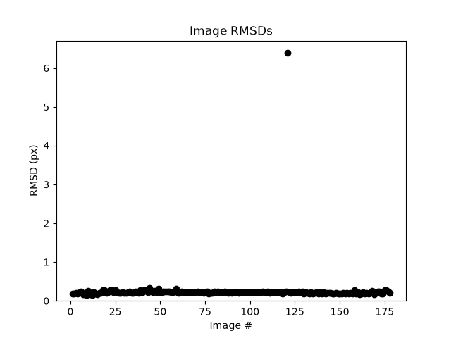
Per-image centroid RMSDs
metric |
value |
|---|---|
images refined |
178 of 179 |
images with RMSD < 1 px |
177 of 178 |
median RMSD |
0.22 px |
outlier |
image 121, RMSD 6.40 px |
refined unit cell (Å) |
a = 34.301 ± 0.006, b = 45.538 ± 0.025, c = 98.957 ± 0.05 |
The result is a clean bimodal split: 177 of the 178 refined images land at an RMSD of a few tenths of a pixel (median 0.22 px), while a single image (image 121) is a clear outlier at 6.4 px — almost certainly a case where pinkIndexer converged on the wrong candidate lattice. The refined unit cells of the well-indexed images agree with each other to within a few thousandths of an Ångstrom (a ≈ 34.301 ± 0.006, b ≈ 45.538 ± 0.025, c ≈ 98.957 ± 0.05 Å).
A real pipeline would typically screen outliers like image 121 out
before merging — either with an RMSD cut like the one visible here, or
by relying on careless’s own robust merging to down-weight it. For
this tutorial we deliberately carry every successfully refined image
through to prediction and integration unfiltered, so that what you see
below is the raw output of the pipeline rather than a hand-curated
subset.
One caveat is worth knowing about. laue.optimize_indexing protects
the orientation refinement with a robust outlier filter (a minimum
covariance determinant estimate on the observed and predicted scattering
vectors), and reflections it rejects are written out unindexed and
therefore dropped. On a still whose residuals vary systematically across
the detector, the filter can reject a whole region rather than the whole
image. Those reflections take no part in laue.refine, but they are
not lost: the refined geometry still predicts them, and they are
integrated along with everything else in the next two sections. If you
see this on many images it is a hint that the detector model (distance,
tilt, or beam centre) deserves a closer look.
Spot Prediction
With a refined geometry we can predict where every reflection allowed by
the spectrum and the resolution limit should fall on the detector, not
just the strong ones that spot finding picked out. laue.predict
takes the same wavelength and resolution limits as
laue.optimize_indexing. If the wavelength histogram above turned out
to be narrower than the limits you gave earlier, you can tighten
lam_min/lam_max here to avoid predicting spots at wavelengths
where there is no beam.
The predictor also estimates how likely each prediction is to be observable and removes improbable ones, and discards predictions that fall on masked pixels.
N=12

laue.predict poly_refined.expt poly_refined.refl \
    output.reflections="predicted.refl" \
    output.log="laue.predict.log" \
    wavelengths.lam_min=0.97 \
    wavelengths.lam_max=1.20 \
    reciprocal_grid.d_min=1.4 \
    nproc=$N
import numpy as np
from dxtbx.model.experiment_list import ExperimentListFactory
from dials.array_family import flex

poly_expts = ExperimentListFactory.from_json_file("poly_refined.expt", check_format=False)
pred = flex.reflection_table.from_file("predicted.refl")

per_image = np.array([(pred["id"] == i).count(True) for i in range(len(poly_expts))])
print(f"Predicted reflections: {len(pred)} total across {len(poly_expts)} images "
      f"(mean {per_image.mean():.0f} per image)")
metric |
value |
|---|---|
predicted reflections |
320,713 |
images |
178 |
mean per image |
1,802 |
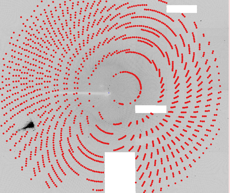
About 1,800 reflections are predicted per image on average, roughly four
times the number of strong spots. The screenshot below shows this for
the first image (predictions are drawn using xyzcal.px, the same
field the viewer uses for any reflection table that has been predicted
or integrated).
dials.image_viewer poly_refined.expt predicted.refl brightness=60
Predicted reflections on the first image
Compare this to the indexed-spots screenshot from the monochromatic-indexing section: there, only a sparse subset of spots along each streak carried a Miller index. Here, after full polychromatic refinement, a prediction lands on essentially every point along every streak — including the weak reflections between the strong spots that spot finding never picked up.
Integration
laue.integrate measures an intensity for every predicted reflection.
For each image it chooses an integration radius from the spacing of the
predicted centroids, pools the pixels of the nearest strong spots to
learn an elliptical profile, and then fits that profile plus a flat
background to the pixels around each prediction. Weak reflections thus
inherit a well-determined profile from their neighbours instead of
fitting noise. The result is written straight to an .mtz file.
N=12

laue.integrate poly_refined.expt predicted.refl \
    output.filename="integrated.mtz" \
    output.log="laue.integrate.log" \
    nproc=$N
The .mtz is unmerged and contains one record per integrated
reflection. We can inspect it with reciprocalspaceship:
import reciprocalspaceship as rs

ds = rs.read_mtz("integrated.mtz")
print(ds.spacegroup.short_name(), ds.cell)
print("Columns:", list(ds.columns))
print("Reflections:", len(ds))
print("Images (batches):", ds["BATCH"].nunique())
ds.head()
The columns are:
column |
meaning |
|---|---|
|
Miller indices |
|
the image number, used by
|
|
integrated intensity and its uncertainty |
|
predicted detector position in pixels |
|
assigned wavelength in Å |
|
fitted background under the spot and its uncertainty |
|
partiality flag unpacked from the
MTZ |
A quick look at the data quality:
import numpy as np
import matplotlib.pyplot as plt
import reciprocalspaceship as rs

ds = rs.read_mtz("integrated.mtz")
ds = ds.compute_dHKL()
d = ds["dHKL"].to_numpy(dtype=float)
isigi = (ds["I"] / ds["SIGI"]).to_numpy(dtype=float)
w = ds["wavelength"].to_numpy(dtype=float)
print("Resolution range: %.2f - %.2f Angstrom" % (d.max(), d.min()))
print("Mean I/sigma(I): %.2f;  fraction with I/sigma(I) > 2: %.2f" % (isigi.mean(), (isigi > 2).mean()))

# Resolution bins with equal volume in reciprocal space
edges = np.linspace(1 / 6.0**3, 1 / d.min() ** 3, 11) ** (-1 / 3)
mids, means = [], []
for hi, lo in zip(edges[:-1], edges[1:]):
    sel = (d <= hi) & (d > lo)
    mids.append(0.5 * (hi + lo))
    means.append(isigi[sel].mean())

fig, axes = plt.subplots(1, 3, figsize=(13, 3.8))
axes[0].plot(1 / np.array(mids) ** 2, means, "o-")
ticks = [6, 4, 3, 2.5, 2, 1.7]
axes[0].set_xticks([1 / t**2 for t in ticks], [str(t) for t in ticks])
axes[0].set_xlabel("Resolution (Å)")
axes[0].set_ylabel("Mean I/σ(I)")
axes[0].set_title("Signal versus resolution")
axes[1].hist(np.clip(isigi, -5, 40), bins=60)
axes[1].set_xlabel("I/σ(I)")
axes[1].set_ylabel("Reflections")
axes[1].set_title("I/σ(I) distribution")
axes[2].hist2d(w, 1 / d**2, bins=[40, 40], cmap="Blues")
axes[2].set_yticks([1 / t**2 for t in ticks], [str(t) for t in ticks])
axes[2].set_xlabel("Wavelength (Å)")
axes[2].set_ylabel("Resolution (Å)")
axes[2].set_title("Integrated reflections")
fig.tight_layout()
fig.savefig("tutorial_images/integrated_stats.png", dpi=130)
plt.show()
Integrated intensity statistics
metric |
value |
|---|---|
space group |
P2₁2₁2₁ |
unit cell (Å) |
34.30, 45.54, 98.96, 90, 90, 90 |
integrated reflections |
317,633 |
resolution range |
49.5 – 1.57 Å |
mean I/σ(I) |
4.5 |
fraction I/σ(I) > 2 |
0.38 |
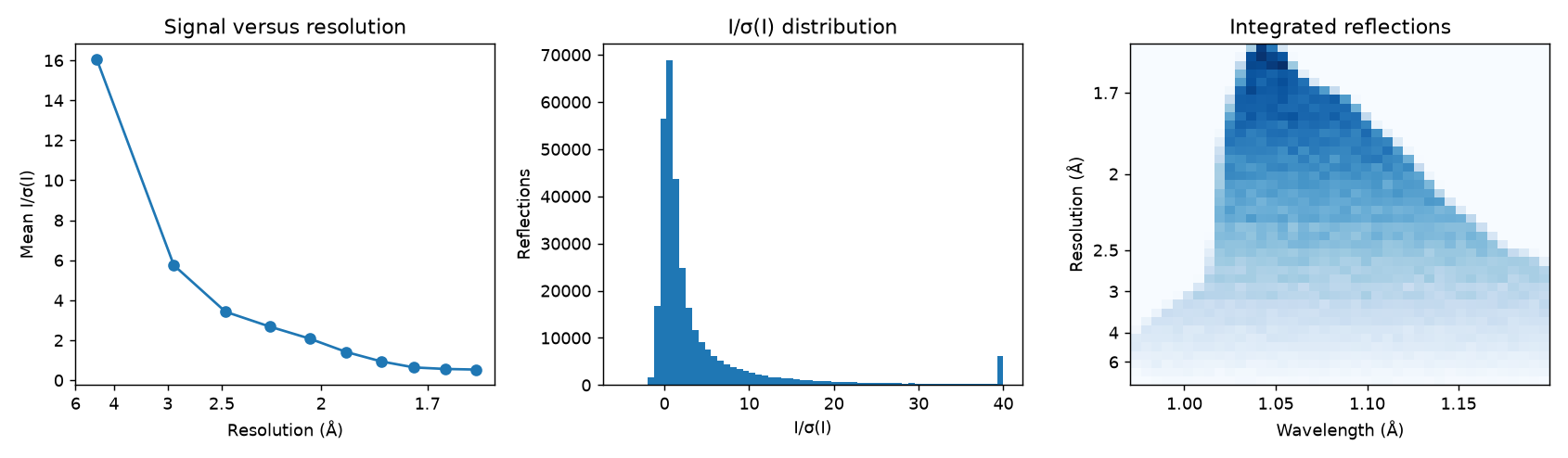
Across the full 179-image collection, laue.integrate produced
317,633 integrated reflections spanning 49.5–1.57 Å, with a mean I/σ(I)
of 4.5 and 38 % of reflections above I/σ(I) = 2. The mean I/σ(I) falls
smoothly with resolution, and the wavelength–resolution plot shows the
full spectrum contributing at every resolution, with most reflections
near the 1.04 Å peak.
Conclusion
At this point you have an integrated, unmerged integrated.mtz
covering all 179 stills (178 of which produced a refined crystal model).
In a real serial experiment you would pass the resulting file(s) to
`careless <https://github.com/rs-station/careless>`__ for scaling
and merging, typically after collecting many more images than this to
compensate for the fraction that fail to index or refine well. Because
the wavelength of every reflection is known, careless is run in
poly mode and given the wavelength column as a metadata key, for
example:
careless poly \
    --iterations=30000 \
    --dmin=1.57 \
    --merge-half-datasets \
    --wavelength-key='wavelength' \
    "xcal,ycal,wavelength,dHKL,BATCH" \
    integrated.mtz \
    merged/dhfr
Every image in a serial run is processed identically, so scaling up further (more images, more crystals) is only a matter of compute time.
Throughout the pipeline you can use DIALS utilities like
dials.image_viewer or dials.report to check progress. Files are
generally written in pairs with the same base name
(poly_refined.expt + poly_refined.refl), with the exception of
imported.expt + strong.refl and poly_refined.expt +
predicted.refl.
Every laue-dials program prints a help page when run without
arguments, and laue.optimize_indexing -c (for example) lists all of
its configurable parameters. The same goes for laue.index -c -e 2,
which is the quickest way to see all of the pinkIndexer options.
Congratulations! This tutorial is now over. For further questions, feel free to consult the documentation or email the authors.