Installation

The easiest way to install laue-dials and its dependencies is using Anaconda. First we update and install the libmamba solver with

conda update -n base conda
conda install -n base conda-libmamba-solver
conda config --set solver libmamba

With Anaconda, we can then create and activate a custom environment for your install by running

conda create --name laue-dials
conda activate laue-dials

Now we are ready to install the main dependency and framework: DIALS. After installing that, we can install laue-dials using pip, as below:

conda install -c conda-forge dials
pip install laue-dials

All other dependencies will then be automatically installed for us, and we’ll be ready to analyze your first Laue data set! Reopen this notebook with the appropriate environment activated when ready.

Documentation for laue-dials can be found at here, and entering a command with no arguments on the command line will also print a help page!

Introduction

In this notebook, we will process a time-resolved EF-X dataset.

The data is comprised of four passes of four timepoints each. Each of the four electric-field timepoints is taken for a given phi angle, then the crystal is rotated around the phi goniometer axis and then the four timepoints are taken again. This is done over four passes, c,d,e,f. The start angle and the step can be found in the below table.

pass	start phi angle (deg)	rotation phi step (deg)
c	0	2
d	92	2
e	181	2
f	361.5	1

At the end of processing, we would like four .mtz files, one for each timepoint. We must run laue-dials on each timepoint individually, then combine all passes for a given timepoint at the end. We start with the off timepoint pass c only. Then, we will analyze all sixteen passes in a single script, and combine the output mtzs into a single mtz file.

Data processing will rely on images found in ./data that can be downloaded on SBGrid and scripts found in ./scripts downloadable here.

Importing Data

We can use dials.import as a way to import the data files written at experimental facilities into a format that is friendly to both DIALS and laue-dials. Feel free to use any data set you’d like below, but a sample time-resolved EF-X data set has been uploaded to Zenodo for your convenience, and this notebook has been tested using that dataset.

First, we create two dictionaries, START_ANGLES and OSCS, that respectively map the pass names to the start angles and rotation steps (treated as oscillations in dials.import).

declare -A START_ANGLES=( ["c"]=0 ["d"]=92 ["e"]=181 ["f"]=361.5)
declare -A OSCS=( ["c"]=2 ["d"]=2 ["e"]=2 ["f"]=1)

Then, we import the files for the c,off images using dials.import.

#this is the delay time.
TIME="off"
# this is the pass.
pass="c"
FILE_INPUT_TEMPLATE="data/e35${pass}_${TIME}_###.mccd"
# Import data into DIALS files
dials.import geometry.scan.oscillation=${START_ANGLES[$pass]},${OSCS[$pass]}\
    geometry.goniometer.invert_rotation_axis=True \
    geometry.goniometer.axes=0,1,0 \
    geometry.beam.wavelength=1.04 \
    geometry.detector.panel.pixel_size=0.08854,0.08854 \
    input.template=$FILE_INPUT_TEMPLATE \
    output.experiments=imported.expt

Getting an Initial Estimate

After importing our data, the first thing we need to do is get an initial estimate for the experimental geometry. Here, we’ll use some monochromatic algorithms from DIALS to help! This step can be tricky – failure can be due to several causes. In the event of failure, here are a few common causes:

1. The spotfinding gain is either too high or too low. Try looking at the results of dials.image_viewer imported.expt strong.refl and seeing if you have too many (or too few) reflections. Lower gain gives you more spots, but also more likely to give false positives.

2. Supplying the space group or unit cell during indexing can be helpful. When supplying the unit cell, allow for some variation in the lengths of the axes, since the monochromatic algorithms may result in a slightly scaled unit cell depending on the chosen wavelength.

3. You may have intensities that need to be masked. These can come from bad panels or extraneous scatter. You can use dials.image_viewer (described below) to create a mask file for your data, and then provide the spotfinder.lookup.mask="pixels.mask" command below to use that mask during spotfinding.

laue.find_spots imported.expt \
    spotfinder.mp.nproc=8 \
    spotfinder.threshold.dispersion.gain=0.3 \
    spotfinder.filter.max_separation=10

CELL='"65.3,39.45,39.01,90.000,117.45,90.000"' #this is a unit cell of PDZ2 from PDB 5E11

laue.index imported.expt strong.refl \
    indexer.indexing.known_symmetry.space_group=5 \
    indexer.indexing.refinement_protocol.mode=refine_shells \
    indexer.indexing.known_symmetry.unit_cell=$CELL \
    indexer.refinement.parameterisation.auto_reduction.action=fix \
    laue_output.index_only=False

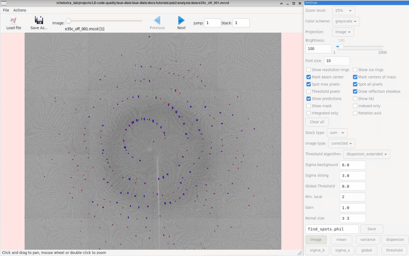
Viewing Images

Sometimes it’s helpful to be able to see the analysis data overlayed on the raw data. DIALS has a utility for viewing spot information on the raw images called dials.image_viewer. For example, the spotfinding gain parameter can be tuned to capture more spots, but lowering it too much finds nonexistent spots. To check this, we can use the image viewer to see what spots were found on images. We need to provide an expt file and a refl file – the imported.expt and strong.refl files will do for checking spotfinding. This program also has utilities for generating masks if they are needed. The red dots from the checkbox “Mark centers of mass” are the spots found by laue.find_spots (which in turn makes a call to dials.find_spots). These are best used for judging whether you need to adjust the gain higher (for fewer spots) or lower (for more) during spotfinding. You can find more details on the image viewer in the DIALS tutorial here.

dials.image_viewer imported.expt strong.refl

Making Stills

Here we will now split our monochromatic estimate into a series of stills to prepare it for the polychromatic pipeline. There is a useful utility called laue.sequence_to_stills for this.

NOTE: Do not use dials.sequence_to_stills, as there are data columns which do not match between the two programs.

laue.sequence_to_stills monochromatic.*

Polychromatic Analysis

Here we will use four other programs in laue-dials to create a polychromatic experimental geometry using our initial monochromatic estimate. Each of the programs does the following:

laue.optimize_indexing assigns wavelengths to reflections and refines the crystal orientation jointly.

laue.refine is a polychromatic wrapper for dials.refine and allows for refining the experimental geometry overall to one suitable for spot prediction and integration.

laue.predict takes the refined experimental geometry and predicts the centroids of all strong and weak reflections on the detector.

laue.integrate then builds spot profiles and integrates intensities on the detector.

laue.optimize_indexing stills.* \
    output.experiments="optimized.expt" \
    output.reflections="optimized.refl" \
    output.log="laue.optimize_indexing.log" \
    wavelengths.lam_min=0.95 \
    wavelengths.lam_max=1.2 \
    reciprocal_grid.d_min=1.7 \
    nproc=8

laue.refine optimized.* \
    output.experiments="poly_refined.expt" \
    output.reflections="poly_refined.refl" \
    output.log="laue.poly_refined.log" \
    nproc=8 >> sink.log

To check the refinement quality, we check the spotfinding root-mean-square deviations (rmsds) as a function of image.

laue.compute_rmsds poly_refined.* refined_only=True show=True save=True

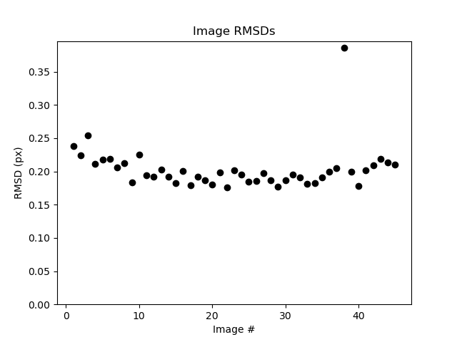
These rmsds look good.

Checking the Wavelength Spectrum

laue.plot_wavelengths allows us to plot the wavelengths assigned in stored in a reflection table. The histogram of these reflections should resemble the beam spectrum, so this is a good check to do at this time!

laue.plot_wavelengths poly_refined.refl refined_only=True save=True show=True

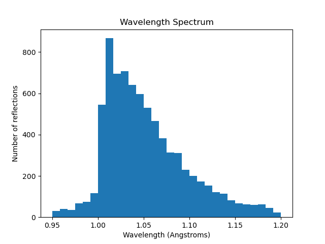
This is the expected wavelength profile, indicating successful wavelength assignment.

DIALS Reports

DIALS has a utility that gives useful information on various diagnostics you may be interested in while analyzing your data. The program dials.report generates an HTML file you can open to see information and plots regarding the status of your analyzed data. You can run it on any files generated by DIALS or laue-dials.

dials.report poly_refined.expt poly_refined.refl

Integrating Spots

Now that we have a refined experiment model, we can use laue.predict and laue.integrate to get integrated intensities from the data. We will predict the locations of all feasible spots on the detector given our refined experiment model, and at each of those locations we will integrate the intensities to get an mtz file that we can feed into careless.

laue.predict poly_refined.* \
    output.reflections="predicted.refl" \
    output.log="laue.predict.log" \
    wavelengths.lam_min=0.95 \
    wavelengths.lam_max=1.2 \
    reciprocal_grid.d_min=1.7 \
    nproc=8

laue.integrate poly_refined.expt predicted.refl \
    output.filename="integrated.mtz" \
    output.log="laue.integrate.log" \
    nproc=8

Processing and Combining All Passes

We have successfully integrated one of the sixteen image series. Let’s now process the rest. For the off timepoints, we process as above. Pass e has a different indexing solution (up to the C2 symmetry operation -x,y,-z) and so we reindex pass e using dials.reindex.

Our strategy for the 50ns,100ns,200ns timepoints is to transfer the stills.expt geometry and then refine spot positions that may have changed due to the electric field.

Using the attached ../scripts/one-pass-from_off.sh script which contains all of the above bash code, we iterate over all of the passes in the below cell. The below cell takes a while to run – we don’t recommend to run this in the jupyter notebook. Instead, we recommend to run it as a standalone parallel script, attached as ../scripts/process.sh. Either procedure will create a folder named gain_0,3 containing subfolders of dials files for each pass. For example, ../gain_0,3-from_stills/dials_files_d_100ns contains dials files for pass d, timepoint 100ns.

declare -A START_ANGLES=( ["c"]=0 ["d"]=92 ["e"]=181 ["f"]=361.5)
declare -A OSCS=( ["c"]=2 ["d"]=2 ["e"]=2 ["f"]=1)
declare -A DELAY="off"

gain=0.3
for pass in c d e f
do
    if [ pass == e ];then
        sh scripts/one_pass-from_off.sh $pass $DELAY ${START_ANGLES[$pass]} ${OSCS[$pass]} $gain -x,y,-z >> sink.log
    else
        sh scripts/one_pass-from_off.sh $pass $DELAY ${START_ANGLES[$pass]} ${OSCS[$pass]} $gain x,y,z >> sink.log
    fi
done

Once the off timepoint series finish, we process the remaining timepoints.

declare -A START_ANGLES=( ["c"]=0 ["d"]=92 ["e"]=181 ["f"]=361.5)
declare -A OSCS=( ["c"]=2 ["d"]=2 ["e"]=2 ["f"]=1)
gain=0.3
for delay in "50ns" "100ns" "200ns"
do
    for pass in "c" "d" "e" "f"
    do
        sh scripts/one_pass-from_off.sh $pass $delay ${START_ANGLES[$pass]} ${OSCS[$pass]} $gain x,y,z >> sink.log
    done
done

Finally, we combine all .mtz files for passes of a single timepoint using the attached scripts/expt_concat.py script. .mtz files can be found in gain_0,3-from_stills/ld_0,3_mtzs.

python scripts/expt_concat.py 0.3

import reciprocalspaceship as rs
rs.read_mtz("gain_0,3/ld_0,3_mtzs/cdef_e35_off.mtz")

We expect a mtz file with about 350,000 reflections.

Conclusion

At this point, you now have integrated mtz files that you can pass to careless for scaling and merging. We provide an example careless script, found at ../scripts/careless-cdef-ohp-mlpw.sh. However, after all Laue-DIALS files are printed out, ../scripts/reduce.sh can also be run for a complete analysis.

Note that throughout this pipeline, you can use DIALS utilities like dials.image_viewer or dials.report to check progress and ensure your data is being analyzed properly. We recommend regularly checking the analysis by looking at the data on images, which can be done by

dials.image_viewer FILE.expt FILE.refl.

These files are generally written as pairs with the same base name, with the exception of combining imported.expt + strong.refl, or poly_refined.expt + predicted.refl.

Also note that you can take any program and enter it on the command-line for further help. For example, writing

laue.optimize_indexing

will print a help page for the program. You can see all configurable parameters by using

laue.optimize_indexing -c.

This applies to all laue-dials command-line programs.

Congratulations! This tutorial is now over. For further questions, feel free to consult documentation or email the authors.